7-11
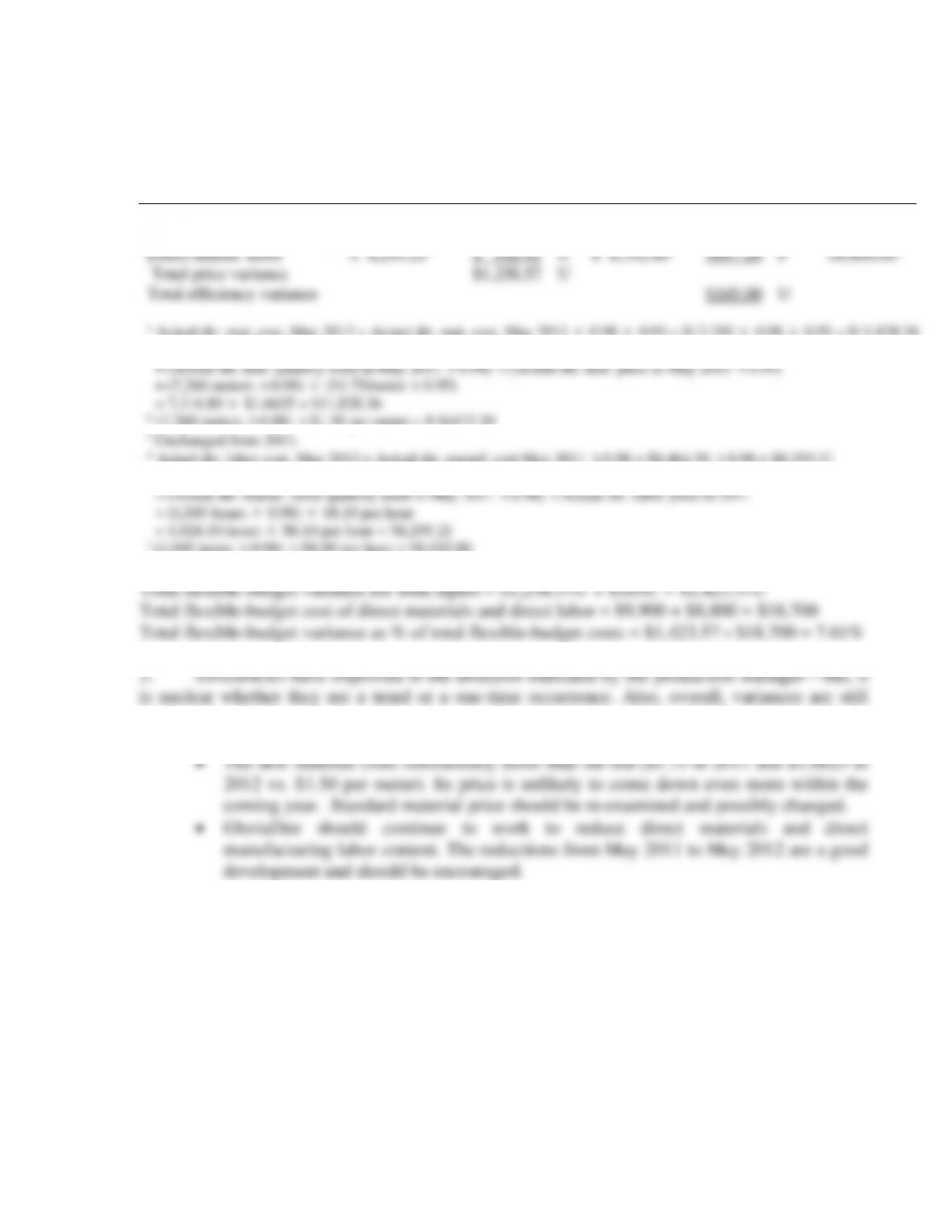
2.
May
2012
Actual
Results
Price
Variance
Actual
Quantity
Budgeted
Price
Efficiency
Variance
Flexible
Budget
(1)
(2) = (1) – (3)
(3)
(4) = (3) – (5)
(5)
Units
550
550
Direct materials
$11,828.36a
$1,156.16
U
$10,672.20b
$772.20
U
$9,900.00c
Direct manuf. labor
$ 8,295.21d
$ 102.41
U
$ 8,192.80e
$607.20
F
$8,800.00c
Total price variance
$1,258.57
U
Total efficiency variance
$165.00
U
0.98
0.95 = $12,705
0.98
0.95 = $11.828.36
Alternatively, actual dir. mat. cost, May 2012
0.98)
$1.50 per meter = $10,672.20
0.98 = $8,464.50
0.98 = $8,295.21
Alternatively, actual dir. labor cost, May 2012
0.98)
$8.00 per hour = $8,192.80
7.6% of flexible input budget. GloriaDee should continue to use the new material, especially in
light of its superior quality and feel, but it may want to keep the following points in mind:
7-12
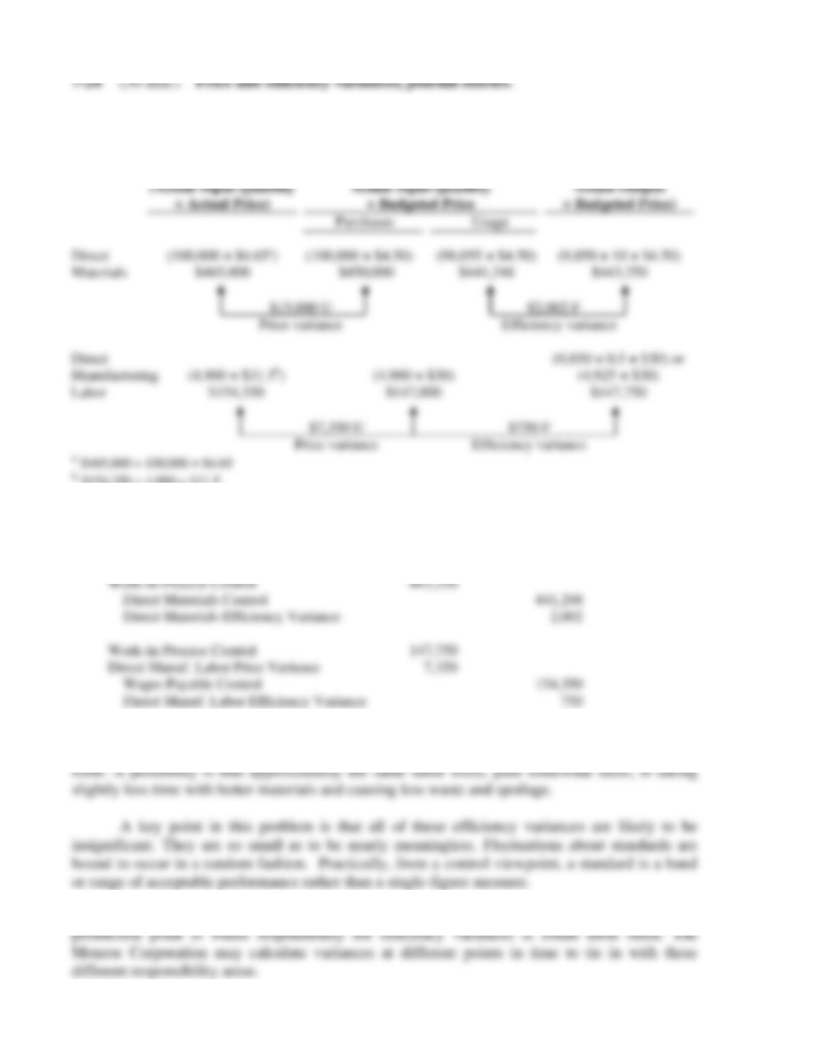
1. Direct materials and direct manufacturing labor are analyzed in turn:
Actual Costs
Incurred
(Actual Input Quantity
× Actual Price)
Actual Input Quantity
× Budgeted Price
Flexible Budget
(Budgeted Input
Quantity Allowed for
Actual Output
× Budgeted Price)
Direct
Materials
(100,000 × $4.65a)
$465,000
Purchases Usage
(100,000 × $4.50) (98,055 × $4.50)
$450,000 $441,248
(9,850 × 10 × $4.50)
$443,250
$15,000 U $2,002 F
Price variance Efficiency variance
Direct
Manufacturing
Labor
(4,900 × $31.5b)
$154,350
(4,900 × $30)
$147,000
(9,850 × 0.5 × $30) or
(4,925 × $30)
$147,750
$7,350 U $750 F
Price variance Efficiency variance
a $465,000 ÷ 100,000 = $4.65
b $154,350 ÷ 4,900 = $31.5
2. Direct Materials Control 450,000
Direct Materials Price Variance 15,000
Accounts Payable or Cash Control 465,000
3. Some students’ comments will be immersed in conjecture about higher prices for
materials, better quality materials, higher grade labor, better efficiency in use of materials, and so
4. The purchasing point is where responsibility for price variances is found most often. The
7-13
1. Standard quantity input amounts per output unit are:
Direct
Materials
(pounds)
Direct
Manufacturing Labor
(hours)
January
February (Jan. × 0.98)
March (Feb. × 0.99)
10.000
9.800
9.702
0.500
0.490
0.485
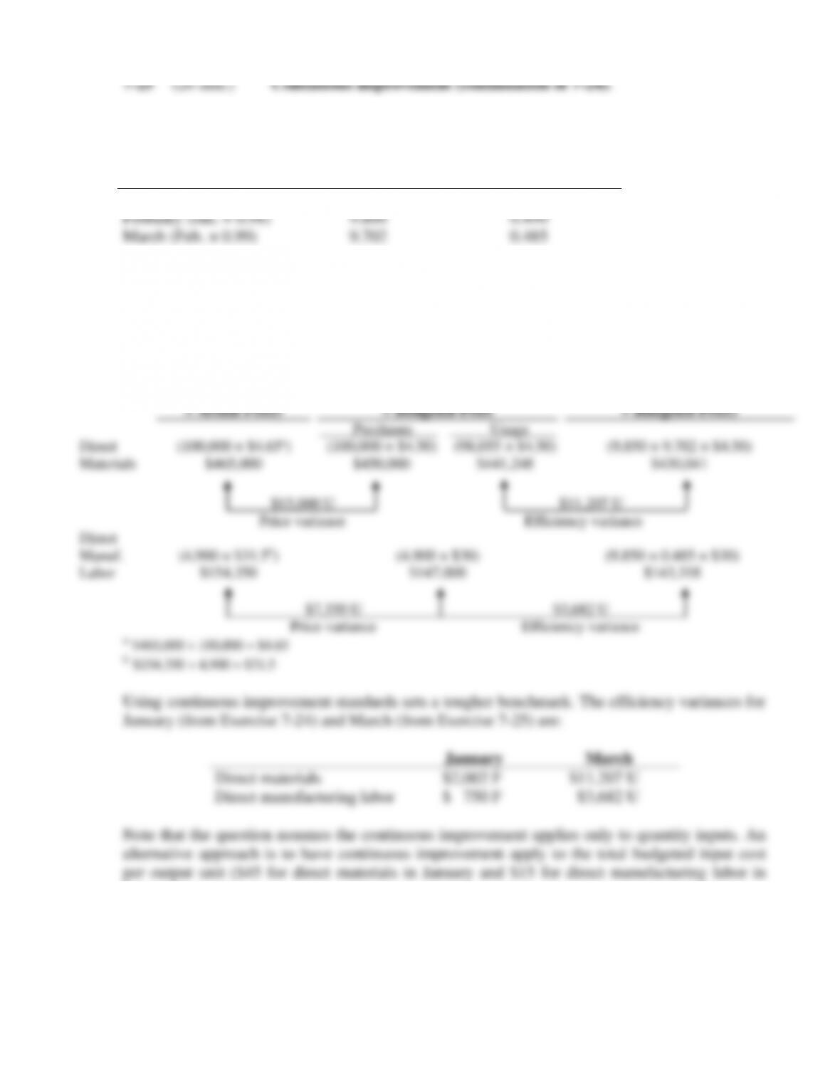
2. The answer is the same as that for requirement 1 of Question 7-24, except for the
flexible-budget amount.
Actual Costs
Incurred
(Actual Input Quantity
× Actual Price)
Actual Input Quantity
× Budgeted Price
Flexible Budget
(Budgeted Input Quantity
Allowed for Actual Output
× Budgeted Price)
Direct
Materials
(100,000 × $4.65a)
$465,000
Purchases Usage
(100,000 × $4.50) (98,055 × $4.50)
$450,000 $441,248
(9,850 × 9.702 × $4.50)
$430,041
$15,000 U $11,207 U
Price variance Efficiency variance
Direct
Manuf.
Labor
(4,900 × $31.5b)
$154,350
(4,900 × $30)
$147,000
(9,850 × 0.485 × $30)
$143,318
$7,350 U $3,682 U
Price variance Efficiency variance
a $465,000 ÷ 100,000 = $4.65
b $154,350 ÷ 4,900 = $31.5
Using continuous improvement standards sets a tougher benchmark. The efficiency variances for
January (from Exercise 7-24) and March (from Exercise 7-25) are:
January
March
Direct materials
Direct manufacturing labor
$2,002 F
$ 750 F
$11,207 U
$3,682 U
Note that the question assumes the continuous improvement applies only to quantity inputs. An
alternative approach is to have continuous improvement apply to the total budgeted input cost
per output unit ($45 for direct materials in January and $15 for direct manufacturing labor in
January).
7-26 (20−30 min.) Materials and manufacturing labor variances, standard costs.
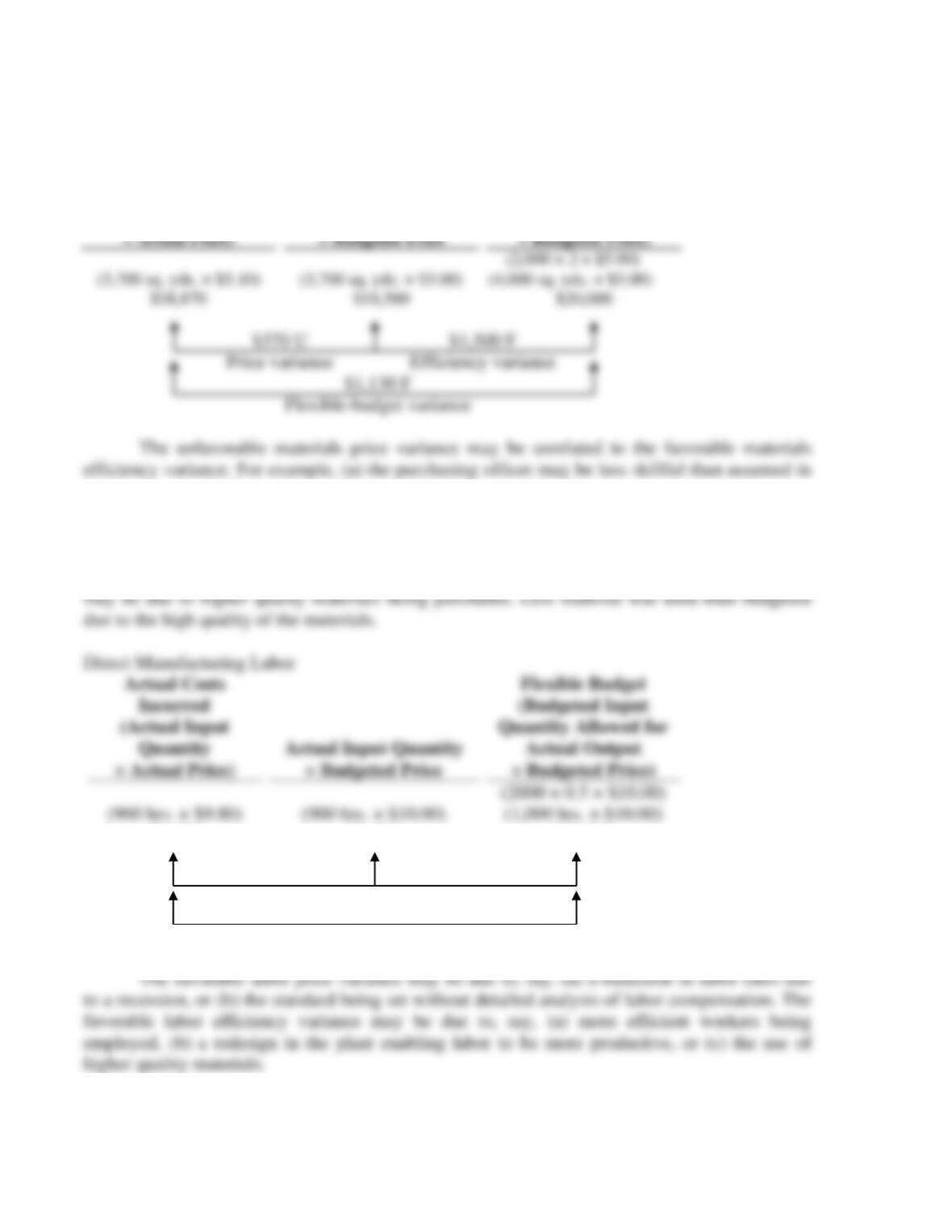
1. Direct Materials
Actual Costs
Incurred
(Actual Input Quantity
× Actual Price)
Actual Input Quantity
× Budgeted Price
Flexible Budget
(Budgeted Input
Quantity Allowed for
Actual Output
× Budgeted Price)
(3,700 sq. yds. × $5.10)
$18,870
(3,700 sq. yds. × $5.00)
$18,500
(2,000 × 2 × $5.00)
(4,000 sq. yds. × $5.00)
$20,000
$370 U $1,500 F
Price variance Efficiency variance
$1,130 F
Flexible-budget variance
The unfavorable materials price variance may be unrelated to the favorable materials
efficiency variance. For example, (a) the purchasing officer may be less skillful than assumed in
the budget, or (b) there was an unexpected increase in materials price per square yard due to
reduced competition. Similarly, the favorable materials efficiency variance may be unrelated to
the unfavorable materials price variance. For example, (a) the production manager may have
been able to employ higher-skilled workers, or (b) the budgeted materials standards were set too
loosely. It is also possible that the two variances are interrelated. The higher materials input price
7-15
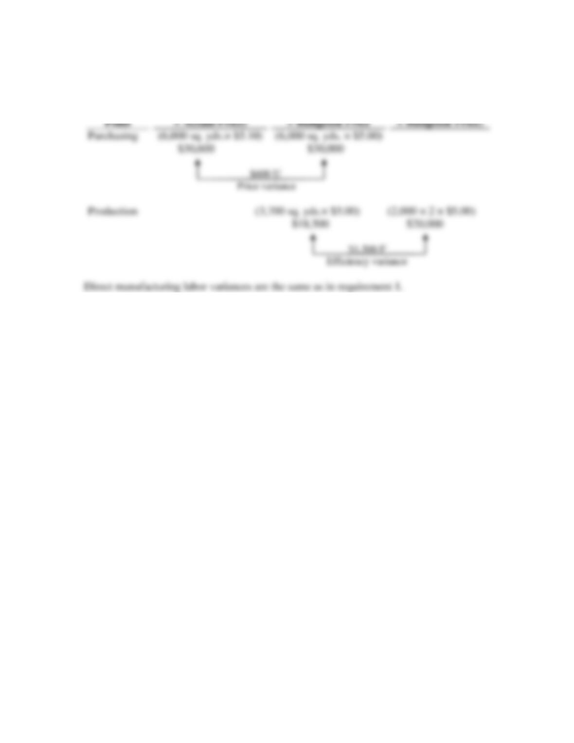
2.
Control
Point
Actual Costs
Incurred
(Actual Input
Quantity
× Actual Price)
Actual Input Quantity
× Budgeted Price
Flexible Budget
(Budgeted Input
Quantity Allowed
for Actual Output
× Budgeted Price)
Purchasing
(6,000 sq. yds.× $5.10)
$30,600
(6,000 sq. yds. × $5.00)
$30,000
$600 U
Price variance
Production
(3,700 sq. yds.× $5.00)
$18,500
(2,000 × 2 × $5.00)
$20,000
$1,500 F
Efficiency variance
Direct manufacturing labor variances are the same as in requirement 1.
7-16
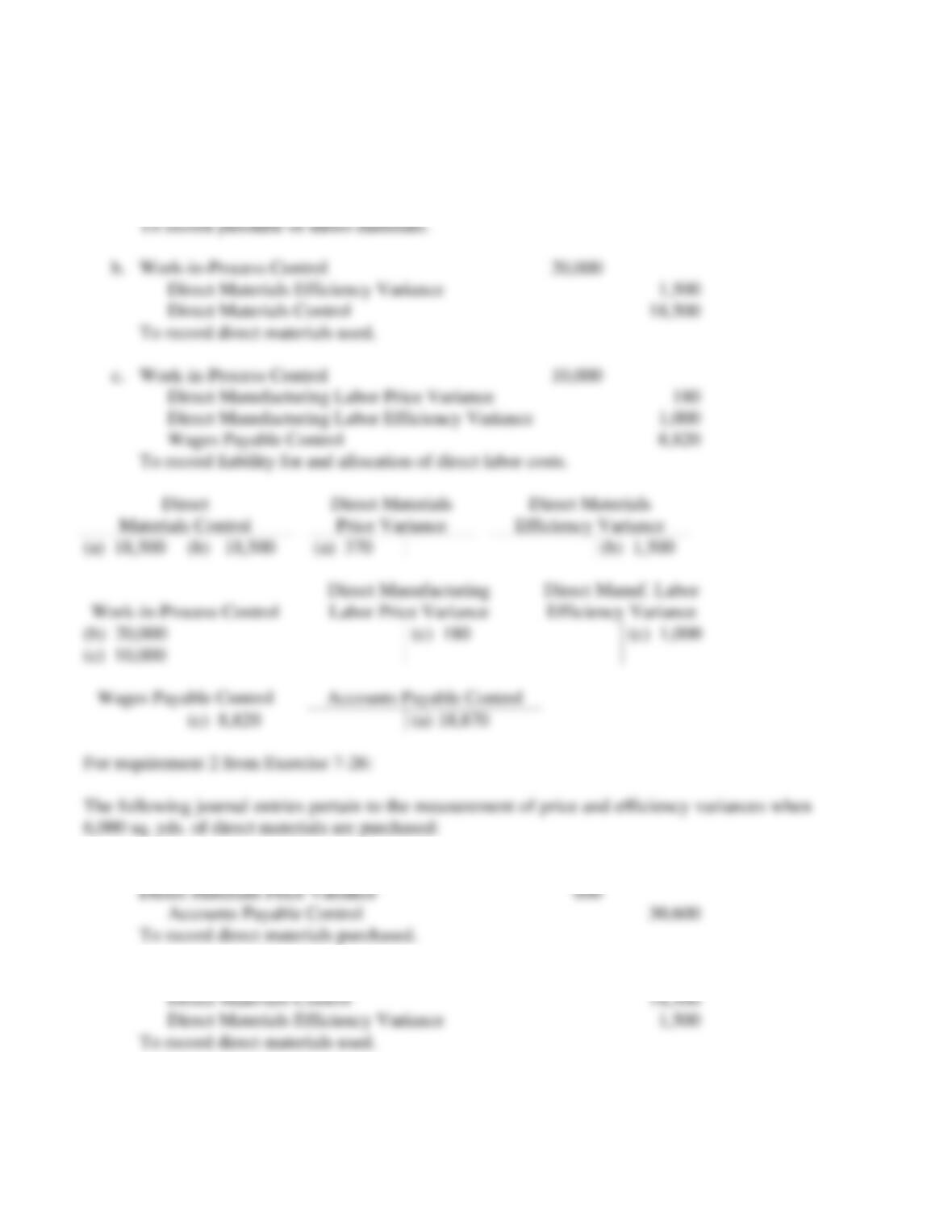
7-27 (15−25 min.) Journal entries and T-accounts (continuation of 7-26).
For requirement 1 from Exercise 7-26:
a. Direct Materials Control 18,500
Direct Materials Price Variance 370
Accounts Payable Control 18,870
a1. Direct Materials Control 30,000
a2. Work-in-Process Control 20,000
7-17
Direct
Materials Control
Direct Materials
Price Variance
(a1) 30,000
(a2) 18,500
(a1) 600
Accounts Payable Control
Work-in–Process Control
(a1) 30,600
(a2) 20,000
Direct Materials
Efficiency Variance
(a2) 1,500
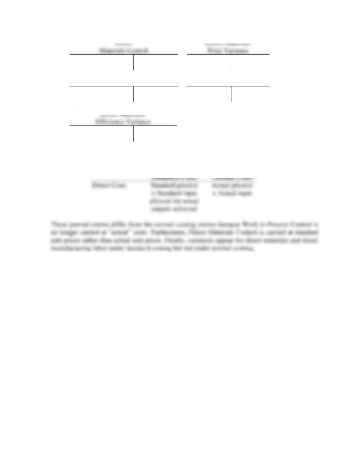
The T–account entries related to direct manufacturing labor are the same as in requirement 1. The
difference between standard costing and normal costing for direct cost items is:
Standard Costs
Normal Costs
Direct Costs
Standard price(s)
× Standard input
allowed for actual
outputs achieved
Actual price(s)
× Actual input
These journal entries differ from the normal costing entries because Work-in-Process Control is
no longer carried at “actual” costs. Furthermore, Direct Materials Control is carried at standard
unit prices rather than actual unit prices. Finally, variances appear for direct materials and direct
manufacturing labor under standard costing but not under normal costing.
7-18
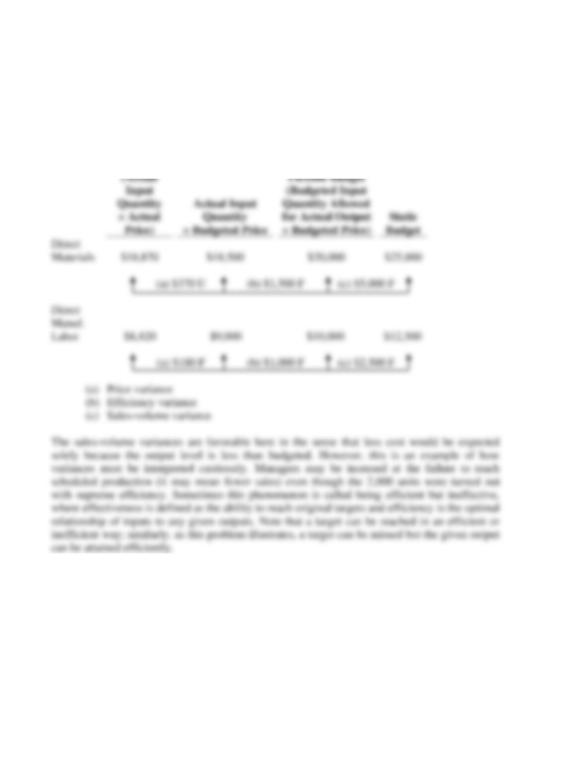
7-28 (25 min.) Flexible budget (Refer to data in Exercise 7-26).
A more detailed analysis underscores the fact that the world of variances may be divided into
three general parts: price, efficiency, and what is labeled here as a sales-volume variance. Failure
to pinpoint these three categories muddies the analytical task. The clearer analysis follows (in
dollars):
Actual Costs
Incurred
(Actual
Input
Quantity
× Actual
Price)
Actual Input
Quantity
× Budgeted Price
Flexible Budget
(Budgeted Input
Quantity Allowed
for Actual Output
× Budgeted Price)
Static
Budget
Direct
Materials
$18,870
$18,500
$20,000
$25,000
(a) $370 U (b) $1,500 F (c) $5,000 F
Direct
Manuf.
Labor
$8,820
$9,000
$10,000
$12,500
(a) $180 F (b) $1,000 F (c) $2,500 F
(a) Price variance
(b) Efficiency variance
(c) Sales-volume variance
The sales-volume variances are favorable here in the sense that less cost would be expected
solely because the output level is less than budgeted. However, this is an example of how
variances must be interpreted cautiously. Managers may be incensed at the failure to reach
scheduled production (it may mean fewer sales) even though the 2,000 units were turned out
with supreme efficiency. Sometimes this phenomenon is called being efficient but ineffective,
where effectiveness is defined as the ability to reach original targets and efficiency is the optimal
relationship of inputs to any given outputs. Note that a target can be reached in an efficient or
inefficient way; similarly, as this problem illustrates, a target can be missed but the given output
can be attained efficiently.
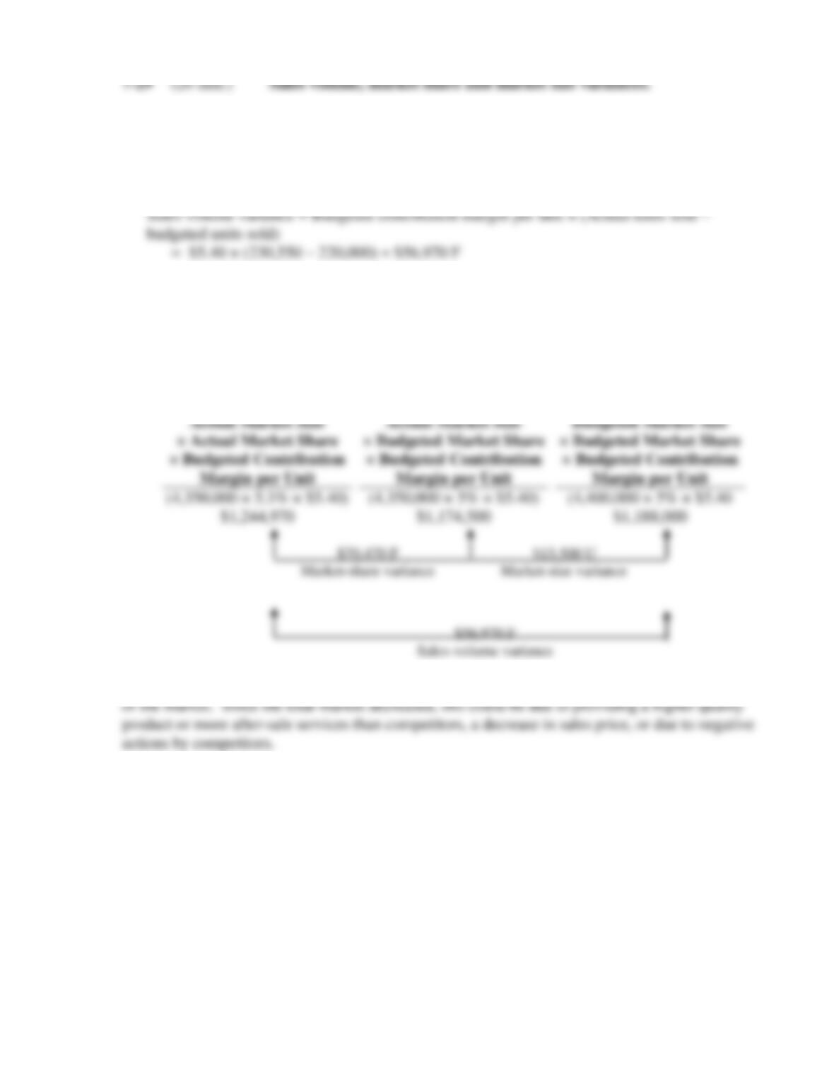
1. Sales volume variance.
Budgeted contribution margin per unit = ($3,300,000 ÷ 220,000) × (1 – 64%) = $5.40
per unit
2. Market share and market size variances
Budgeted market share = 220,000 ÷ 4,400,000 = 5%
Actual market share = 230,550 ÷ 4,350,000 = 5.30%
Actual Market Size
× Actual Market Share
× Budgeted Contribution
Margin per Unit
Actual Market Size
× Budgeted Market Share
× Budgeted Contribution
Margin per Unit
Static Budget:
Budgeted Market Size
× Budgeted Market Share
× Budgeted Contribution
Margin per Unit
(4,350,000 × 5.3% × $5.40)
$1,244,970
(4,350,000 × 5% × $5.40)
$1,174,500
(4,400,000 × 5% × $5.40
$1,188,000
$70,470 F $13,500 U
Market-share variance Market-size variance
3. The market share variance is favorable indicating that the company increased its percentage
$56,970 F
Sales-volume variance
7-20
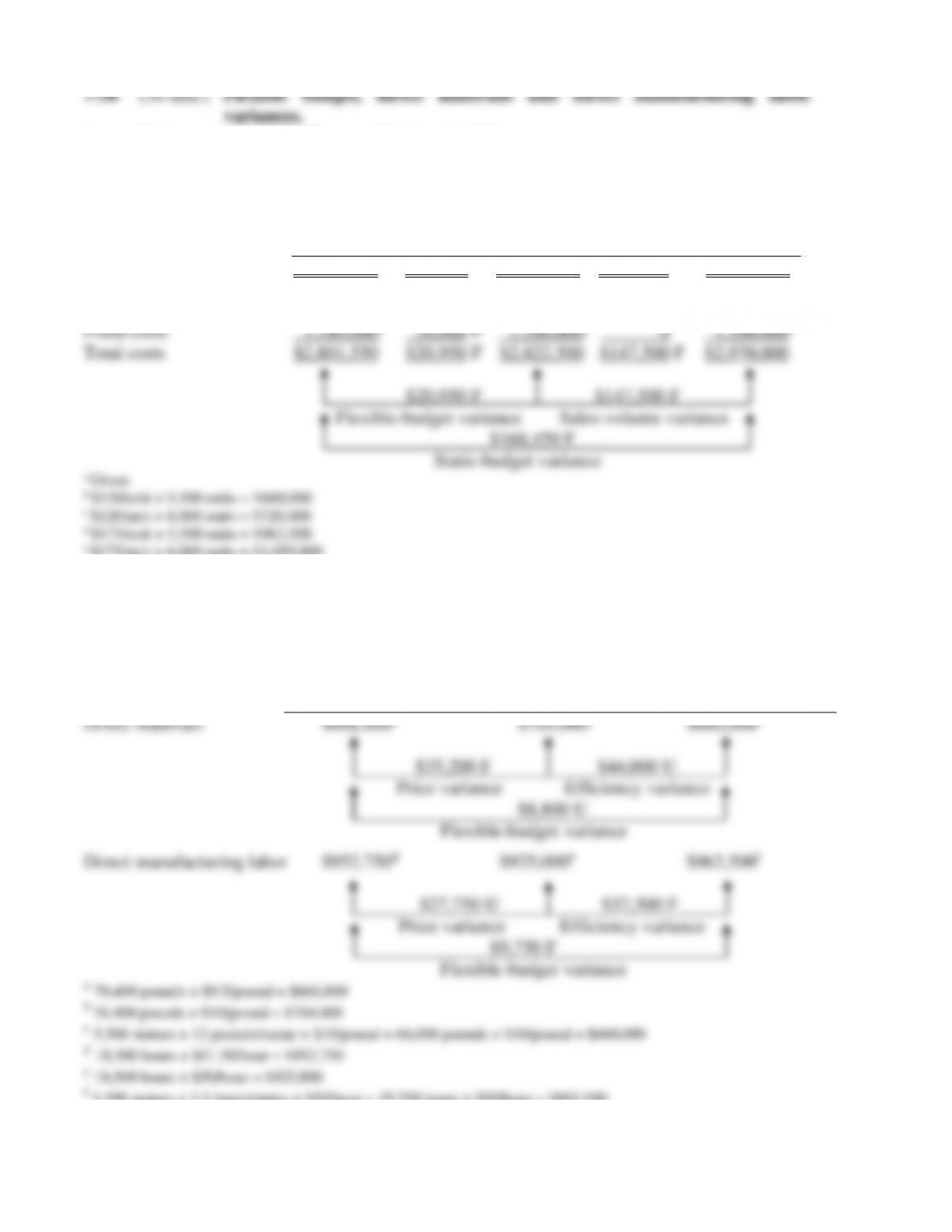
1. Variance Analysis for Tuscany Statuary for 2011
Actual
Results
(1)
Flexible
Budget
Variances
(2) = (1) – (3)
Flexible
Budget
(3)
Sales
Volume
Variances
(4) = (3) – (5)
Static
Budget
(5)
Units sold 5,500a 0 5,500 500 U 6,000a
Direct materials $ 668,800 $ 8,800 U $ 660,000 b $ 60,000 F $ 720,000c
Direct manufacturing labor 952,750a 9,750 F 962,500d 87,500 F 1,050,000e
2.
Actual Incurred
(Actual Input
Quantity
Actual Price)
Actual Input
Quantity
Budgeted Price
Flexible Budget
(Budgeted Input
Quantity Allowed for
Actual Output
Budgeted Price)