7-1
CHAPTER 7
7-1 Management by exception is the practice of concentrating on areas not operating as
7-3 A favorable variance––denoted F––is a variance that has the effect of increasing
7-4 The key difference is the output level used to set the budget. A static budget is based on
7-5 A flexible-budget analysis enables a manager to distinguish how much of the difference
7-6 The steps in developing a flexible budget are:
Step 1: Identify the actual quantity of output.
7-7 Four reasons for using standard costs are:
(i) cost management,
7-8 A manager should subdivide the flexible-budget variance for direct materials into a price
variance (that reflects the difference between actual and budgeted prices of direct materials) and
7-2
7-9 Possible causes of a favorable direct materials price variance are:
• purchasing officer negotiated more skillfully than was planned in the budget,
7-10 Some possible reasons for an unfavorable direct manufacturing labor efficiency variance
are the hiring and use of underskilled workers; inefficient scheduling of work so that the
7-11 Variance analysis, by providing information about actual performance relative to
standards, can form the basis of continuous operational improvement. The underlying causes of
7-12 An individual business function, such as production, is interdependent with other
business functions. Factors outside of production can explain why variances arise in the
7-13 The plant supervisor likely has good grounds for complaint if the plant accountant puts
7-14 The sales-volume variance can be decomposed into two parts: a market-share variance
7-15 Evidence on the costs of other companies is one input managers can use in setting the
performance measure for next year. However, caution should be taken before choosing such an
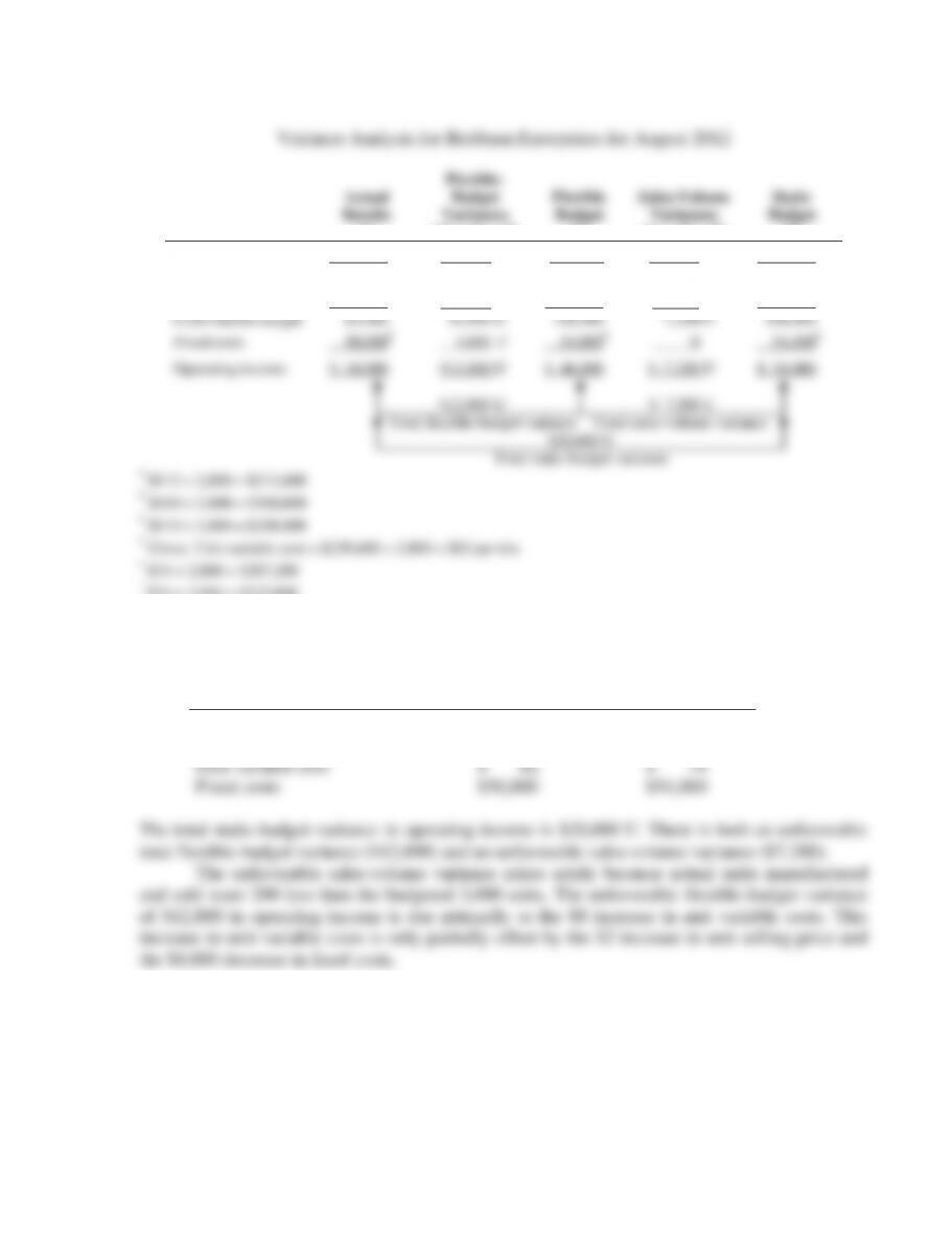
7-16 (20–30 min.) Flexible budget.
Actual
Results
(1)
Flexible-
Budget
Variances
(2) = (1) – (3)
Flexible
Budget
(3)
Sales-Volume
Variances
(4) = (3) – (5)
Static
Budget
(5)
Units (tires) sold
2,800g
0
2,800
200 U
3,000g
Revenues
$313,600a
$ 5,600 F
$308,000b
$22,000 U
$330,000c
Variable costs
229,600d
22,400 U
207,200e
14,800 F
222,000f
Contribution margin
84,000
16,800 U
100,800
7,200 U
108,000
Fixed costs
50,000g
4,000 F
54,000g
0
54,000g
Operating income
$ 34,000
$12,800 U
$ 46,800
$ 7,200 U
$ 54,000
$12,800 U $ 7,200 U
Total flexible-budget variance Total sales-volume variance
$20,000 U
Total static-budget variance
a $112 × 2,800 = $313,600
b $110 × 2,800 = $308,000
c $110 × 3,000 = $330,000
d Given. Unit variable cost = $229,600 ÷ 2,800 = $82 per tire
e $74 × 2,800 = $207,200
f $74 × 3,000 = $222,000
g Given
2. The key information items are:
Actual
Budgeted
Units
Unit selling price
Unit variable cost
Fixed costs
2,800
$ 112
$ 82
$50,000
3,000
$ 110
$ 74
$54,000
The total static-budget variance in operating income is $20,000 U. There is both an unfavorable
total flexible-budget variance ($12,800) and an unfavorable sales-volume variance ($7,200).
The unfavorable sales-volume variance arises solely because actual units manufactured
and sold were 200 less than the budgeted 3,000 units. The unfavorable flexible-budget variance
of $12,800 in operating income is due primarily to the $8 increase in unit variable costs. This
increase in unit variable costs is only partially offset by the $2 increase in unit selling price and
the $4,000 decrease in fixed costs.
7-4
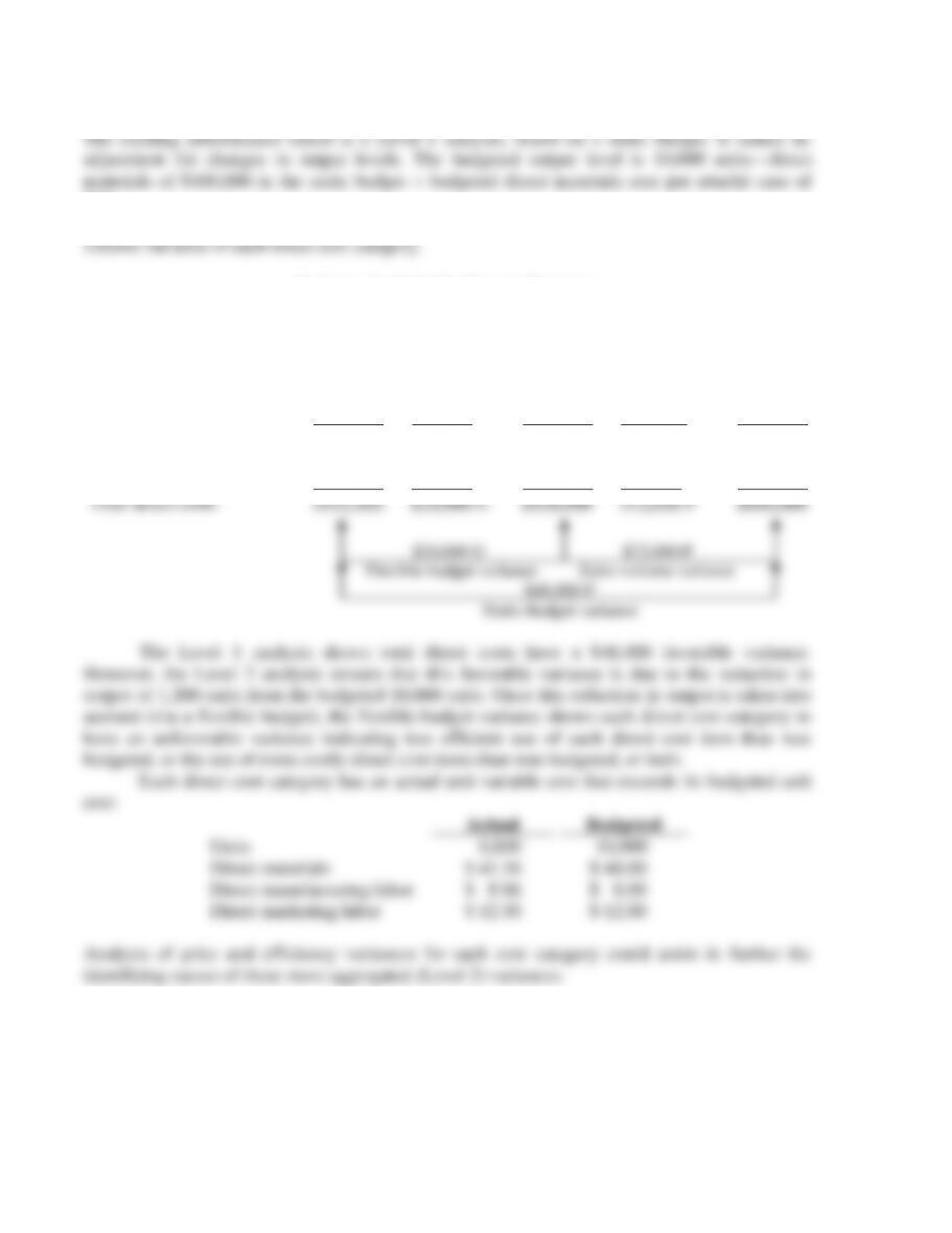
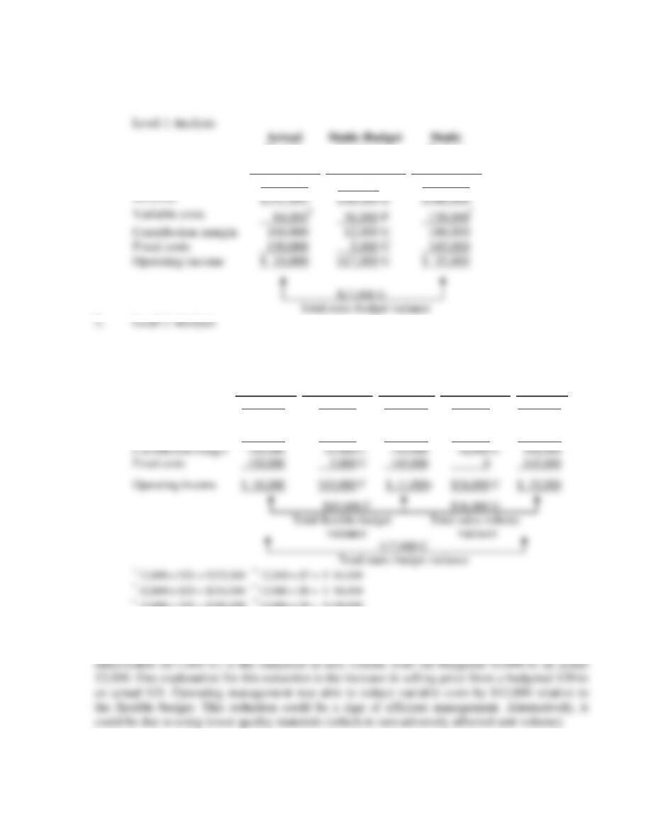
7-17 (15 min.) Flexible budget.
$40.
The following is a Level 2 analysis that presents a flexible-budget variance and a sales-
Actual
Results
(1)
Flexible-
Budget
Variances
(2) = (1) – (3)
Flexible
Budget
(3)
Sales-
Volume
Variances
(4) = (3) – (5)
Static
Budget
(5)
Output units
Direct materials
Direct manufacturing labor
Direct marketing labor
Total direct costs
8,800
$364,000
78,000
110,000
$552,000
0
$12,000 U
7,600 U
4,400 U
$24,000 U
8,800
$352,000
70,400
105,600
$528,000
1,200 U
$48,000 F
9,600 F
14,400 F
$72,000 F
10,000
$400,000
80,000
120,000
$600,000
$24,000 U $72,000 F
Flexible-budget variance Sales-volume variance
$48,000 F
Static-budget variance
The Level 1 analysis shows total direct costs have a $48,000 favorable variance.
However, the Level 2 analysis reveals that this favorable variance is due to the reduction in
output of 1,200 units from the budgeted 10,000 units. Once this reduction in output is taken into
account (via a flexible budget), the flexible-budget variance shows each direct cost category to
have an unfavorable variance indicating less efficient use of each direct cost item than was
budgeted, or the use of more costly direct cost items than was budgeted, or both.
Each direct cost category has an actual unit variable cost that exceeds its budgeted unit
cost:
Actual
Budgeted
Units
Direct materials
Direct manufacturing labor
Direct marketing labor
8,800
$ 41.36
$ 8.86
$ 12.50
10,000
$ 40.00
$ 8.00
$ 12.00
Analysis of price and efficiency variances for each cost category could assist in further the
identifying causes of these more aggregated (Level 2) variances.
7-18 (25–30 min.) Flexible-budget preparation and analysis.
1. Variance Analysis for Bank Management Printers for September 2012
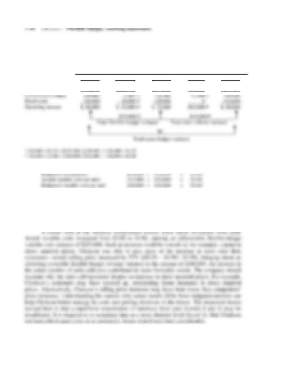
7-6
1. Variance Analysis for The Clarkson Company for the year ended December 31, 2012
Actual
Results
(1)
Flexible-
Budget
Variances
(2)=(1)−(3)
Flexible
Budget
(3)
Sales-Volume
Variances
(4)=(3)−(5)
Static
Budget
(5)
Units sold
130,000
0
130,000
10,000 F
120,000
Revenues
$715,000
$260,000 F
$455,000a
$35,000 F
$420,000
Variable costs
515,000
255,000 U
260,000b
20,000 U
240,000
Contribution margin
200,000
5,000 F
195,000
15,000 F
180,000
Fixed costs
140,000
20,000 U
120,000
0
120,000
Operating income
$ 60,000
$ 15,000 U
$ 75,000
$15,000 F
$ 60,000
2. Actual selling price: $715,000 130,000 = $5.50
3. A zero total static-budget variance may be due to offsetting total flexible-budget and total
sales-volume variances. In this case, these two variances exactly offset each other:
Total flexible-budget variance $15,000 Unfavorable
Total sales-volume variance $15,000 Favorable
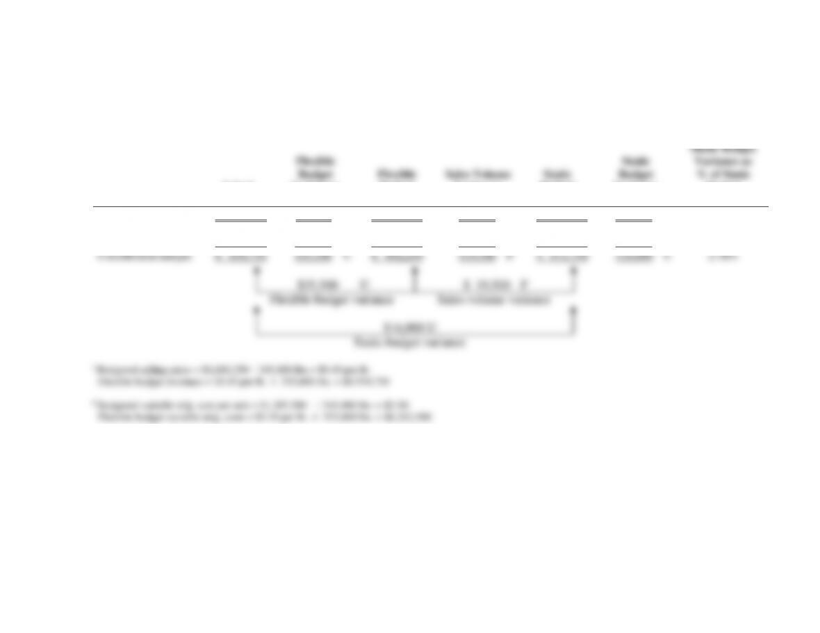
7-20 (30-40 min.) Flexible budget and sales volume variances, market-share and market-size variances.
1. and 2.
Performance Report for Marron, Inc., June 2012
Actual
Flexible
Budget
Variances
Flexible
Budget
Sales Volume
Variances
Static
Budget
Static
Budget
Variance
Static Budget
Variance as
% of Static
Budget
(1)
(2) = (1) – (3)
(3)
(4) = (3) – (5)
(5)
(6) = (1) – (5)
(7) = (6)
(5)
Units (pounds)
355,000
—
355,000
10,000
F
345,000
10,000
F
2.90%
Revenues
$1,917,000
$17,750
U
$1,934,750a
$54,500
F
$1,880,250
$36,750
F
1.95%
Variable mfg. costs
1,260,250
17,750
U
1,242,500b
35,000
U
1,207,500
52,750
U
4.37%
Contribution margin
$ 656,750
$35,500
U
$ 692,250
$19,500
F
$ 672,750
$16,000
U
2.38%
$35,500 U $ 19,500 F
Flexible-budget variance Sales-volume variance
$16,000 U
Static-budget variance
a Budgeted selling price = $1,880,250
345,000 lbs = $5.45 per lb.
Flexible-budget revenues = $5.45 per lb.
355,000 lbs. = $1,934,750
b Budgeted variable mfg. cost per unit = $1,207,500
345,000 lbs. = $3.50
Flexible-budget variable mfg. costs = $3.50 per lb.
355,000 lbs. = $1,242,500
7-8
3. The selling price variance, caused solely by the difference in actual and budgeted selling
price, is the flexible-budget variance in revenues = $17,750 U.
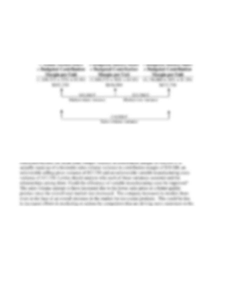
4. Budgeted market share = 345,000 ÷ 1,150,000 = 30%
Actual market share = 355,000 ÷ 1,109,375 = 32%
Actual Market Size
× Actual Market Share
× Budgeted Contribution
Margin per Unit
Actual Market Size
× Budgeted Market Share
× Budgeted Contribution
Margin per Unit
Static Budget:
Budgeted Market Size
× Budgeted Market Share
× Budgeted Contribution
Margin per Unit
(1,109,375 × 32% × $1.95)
$692,250
(1,109,375 × 30% × $1.95)
$648,984
(1,150,000 × 30% × $1.95)
$672,750
$43,266 F $23,766 U
Market-share variance Market-size variance
5. The flexible-budget variances show that for the actual sales volume of 355,000 pounds,
selling prices were lower and costs per pound were higher. The favorable sales volume variance
in revenues (because more pounds of ice cream were sold than budgeted) helped offset the
unfavorable variable cost variance and shored up the results in June 2012. Levine should be more
company.
$19,500 F
Sales-volume variance
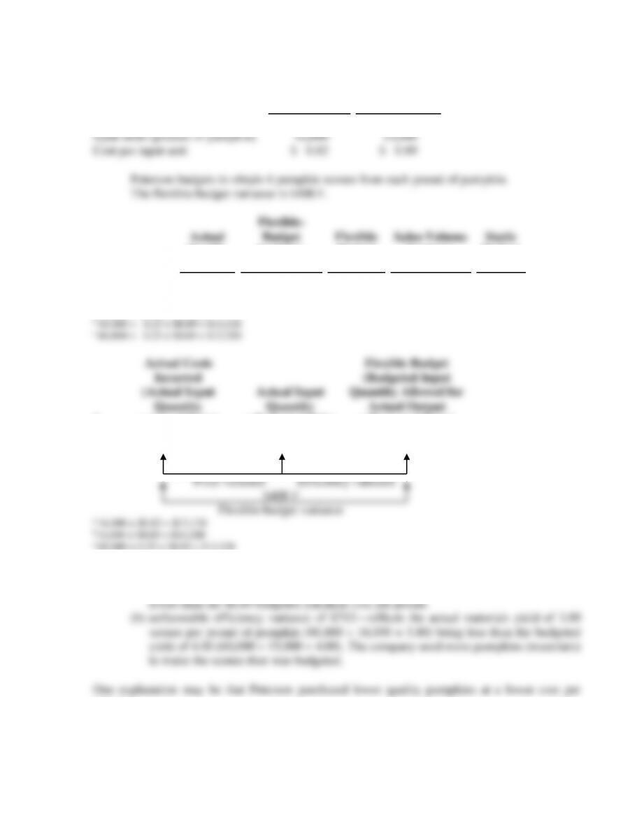
7-21 (20–30 min.) Price and efficiency variances.
1. The key information items are:
Actual
Budgeted
Output units (scones)
Input units (pounds of pumpkin)
Cost per input unit
60,800
16,000
$ 0.82
60,000
15,000
$ 0.89
Peterson budgets to obtain 4 pumpkin scones from each pound of pumpkin.
The flexible-budget variance is $408 F.
Actual
Results
(1)
Flexible-
Budget
Variance
(2) = (1) – (3)
Flexible
Budget
(3)
Sales-Volume
Variance
(4) = (3) – (5)
Static
Budget
(5)
Pumpkin costs
$13,120a
$408 F
$13,528b
$178 U
$13,350c
a 16,000 × $0.82 = $13,120
2.
Actual Costs
Incurred
(Actual Input
Quantity
× Actual Price)
Actual Input
Quantity
× Budgeted Price
Flexible Budget
(Budgeted Input
Quantity Allowed for
Actual Output
× Budgeted Price)
$13,120a
$14,240b
$13,528c
$1,120 F $712 U
3. The favorable flexible-budget variance of $408 has two offsetting components:
(a) favorable price variance of $1,120––reflects the $0.82 actual purchase cost being
pound.
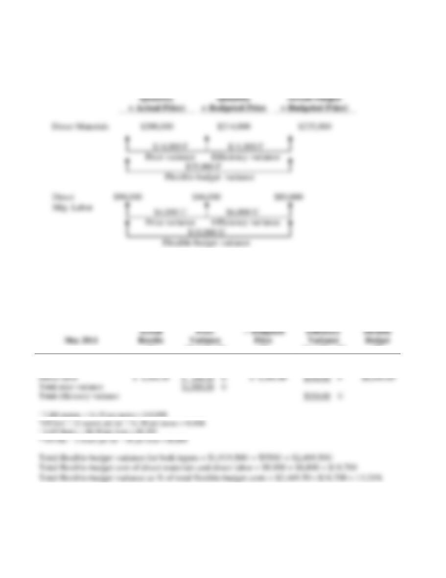
7-22 (15 min.) Materials and manufacturing labor variances.
Actual Costs
Incurred
(Actual Input
Quantity
× Actual Price)
Actual Input
Quantity
× Budgeted Price
Flexible Budget
(Budgeted Input
Quantity Allowed for
Actual Output
× Budgeted Price)
Direct Materials
$200,000
$214,000
$225,000
$14,000 F $11,000 F
Price variance Efficiency variance
$25,000 F
Flexible-budget variance
Direct $90,000 $86,000 $80,000
Mfg. Labor $4,000 U $6,000 U
Price variance Efficiency variance
$10,000 U
Flexible-budget variance
7-23 (30 min.) Direct materials and direct manufacturing labor variances.
1.
May 2011
Actual
Results
Price
Variance
Actual
Quantity
Budgeted
Price
Efficiency
Variance
Flexible
Budget
(1)
(2) = (1)–(3)
(3)
(4) = (3) – (5)
(5)
Units
550
550
Direct materials
$12,705.00
$1,815.00
U
$10,890.00a
$990.00
U
$9,900.00b
Direct labor
$ 8,464.50
$ 104.50
U
$ 8,360.00c
$440.00
F
$8,800.00d
Total price variance
$1,919.50
U
Total efficiency variance
$550.00
U