19-21
19-29 (30–40 min.) Statistical quality control.
1. The + 2 rule will trigger a decision to investigate when mean weight per production run
is outside the control limit:
Double Bran Bits: Mean + 2 = 17.97 + (2 0.28) or 17.41 to 18.53 oz.
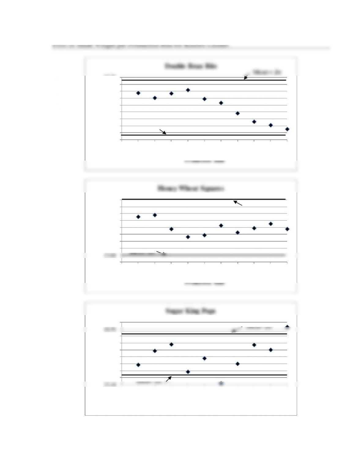
2. Solution Exhibit 19-29 presents the SQC charts for each of the three breakfast cereals.
Double Bran Bits had no observations outside the control limits. Each of the production
runs is considered to be in conformance with quality standards. However, there is an apparent
trend from the SQC that the mean of each of the later production runs gets nearer to the lower
19-22
3. The costs of quality include
(2) Appraisal costs—Costs of inspection to check the weight of cereal boxes.
(3) Internal failure costs—Costs of refilling cereal boxes that do not meet specifications;
(4) External failure costs—Costs of customer ill-will if they discover that cereal boxes
are underfilled, costs of returning and replacing incorrectly filled boxes.
Six sigma quality is a standard of excellence that requires a strict understanding of both
customer expectations and reasons for manufacturing defects to improve current quality
19-23
SOLUTION EXHIBIT 19-29
17.30
17.44
17.58
17.72
17.86
18.00
18.14
18.28
18.42
18.56
0 1 2 3 4 5 6 7 8 9 10
Weight
Production Run
Double Bran Bits
Mean + 2
Mean –2
13.60
13.68
13.76
13.84
13.92
14.00
14.08
14.16
14.24
14.32
0 1 2 3 4 5 6 7 8 9 10
Weight
Production Run
Honey Wheat Squares
Mean+2
Mean–2
15.44
15.58
15.72
15.86
16.00
16.14
16.28
16.42
16.56
16.70
0 1 2 3 4 5 6 7 8 9 10
Weight
Production Run
Sugar King Pops
Mean–2
Mean–2
19-24
19-30 (30–40 min.) Compensation linked with profitability, waiting time, and quality
measures.
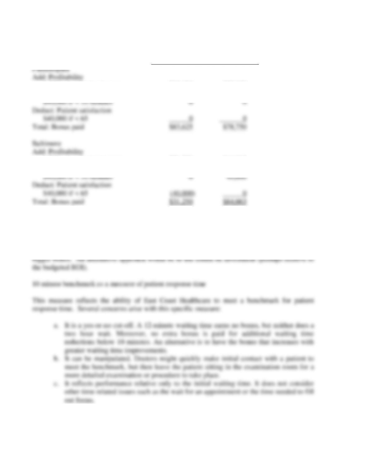
1.
Jan.-June
July-Dec.
Philadelphia
Add: Profitability
0.75% of operating income
$83,625
$78,750
Add: Average waiting time
$40,000 if < 10 minutes
0
0
Deduct: Patient satisfaction
$40,000 if < 65
0
0
Total: Bonus paid
$83,625
$78,750
Baltimore
Add: Profitability
0.75% of operating income
$71,250
$44,063
Add: Average waiting time
$40,000 if < 10 minutes
0
40,000
Deduct: Patient satisfaction
$40,000 if < 65
(40,000)
0
Total: Bonus paid
$31,250
$84,063
2. Operating income as a measure of profitability
Operating income captures revenue and cost-related factors. However, there is no recognition of
investment differences between the two groups. If one group is substantially bigger than the
other, differences in size alone give the president of the larger group the opportunity to earn a
19-25
Problems in (b) and (c) can be overcome by measuring total patient response time (such as how
long it takes from the time a patient makes an appointment to the time the actual appointment is
concluded), in addition to average waiting time to meet the doctor.
Patient satisfaction as a measure of quality
3. Most companies use both financial and nonfinancial measures to evaluate performance,
sometimes presented in a single report such as a balanced scorecard. Using multiple measures of
performance enables top management to evaluate whether lower-level managers have improved
one area at the expense of others. For example, did the better average waiting time (and patient
19-31 (25–30 min.) Waiting times, manufacturing cycle times.
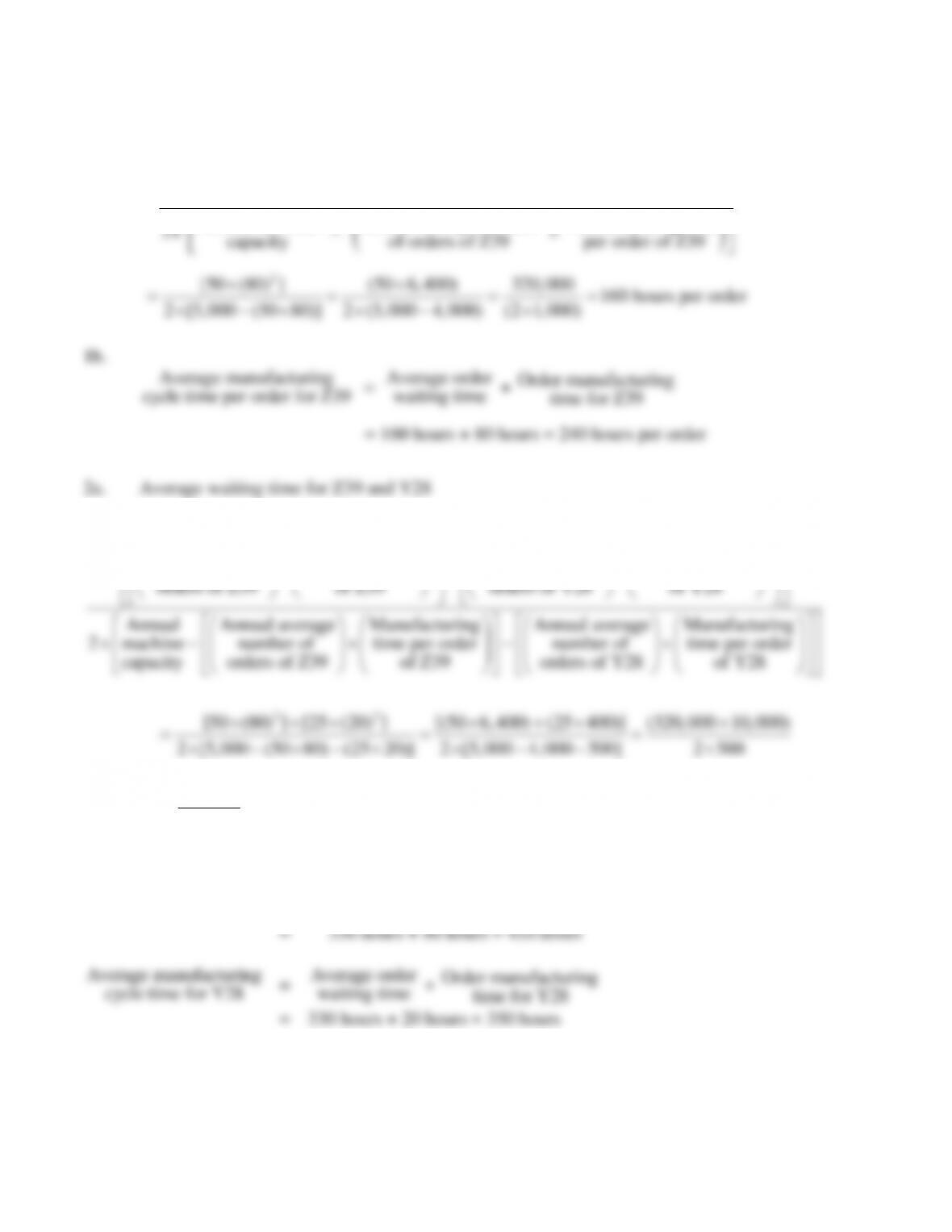
1a. Average waiting time for an order of Z39
( ) ( )
( )
2
Annual average number Manufacturing time
of orders of Z39 per order of Z39
Annual machine Annual average number Manufacturing time
2
capacity of orders of Z39 per order of Z39
x
−
2
[50 (80) ] (50 6,400) 320,000 160 hours per order
2 [5,000 (50 80)] 2 (5,000 4,000) (2 1,000)
= = = =
− −
1b.
Average manufacturing
cycle time per order for Z39
=
Average order
waiting time
+
Order manufacturing
time for Z39
= 160 hours + 80 hours = 240 hours per order
2a. Average waiting time for Z39 and Y28
22
Annual average Manufacturing Annual average Manufacturing
number of time per order number of time per order
orders of Z39 of Z39 orders of Y28 of Y28
Annual Annual average Manufacturing Annual average Manufacturing
2 machine number of time per order number of time per or
capacity orders of Z39 of Z39 orders of Y28
− −
der
of Y28
22
[50 (80) ] [25 (20) ] [(50 6,400) (25 400)] (320,000 10,000)
2 [5,000 (50 80) (25 20)] 2 [5,000 4,000 500] 2
+ + +
= = =
− − − −
330,000 330 hours
1,000
==
2b.
Average manufacturing
cycle time for Z39
=
Average order
waiting time
+
Order manufacturing
time for Z39
Average order
waiting time
19-27
19-32 (60 min.) Waiting times, relevant revenues, and relevant costs
(continuation of 19-31).
1. The direct approach is to look at incremental revenues and incremental costs.
Selling price per order of Y28, which has
an average manufacturing lead time of 350 hours $ 8,000
Variable cost per order 5,000
Additional contribution per order of Y28 3,000
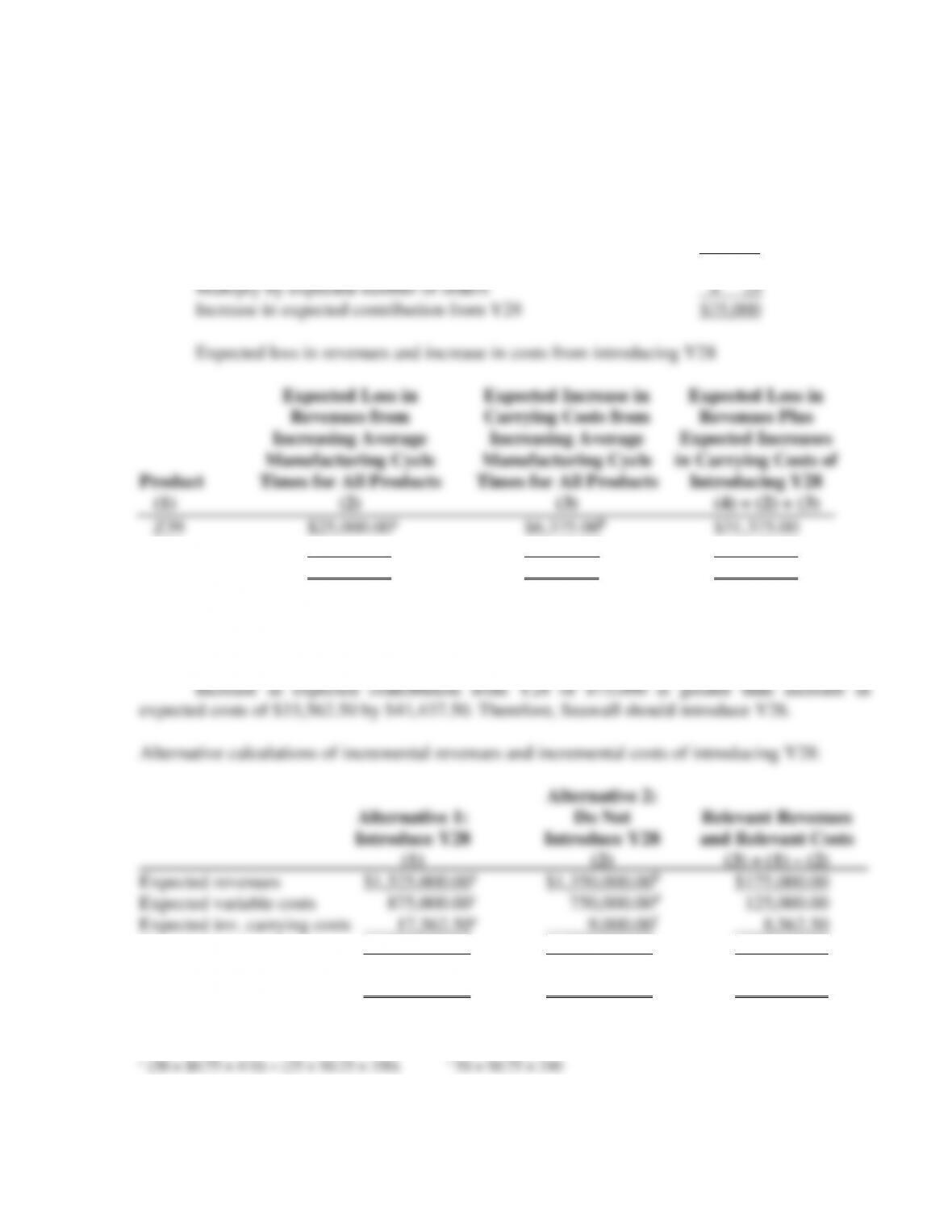
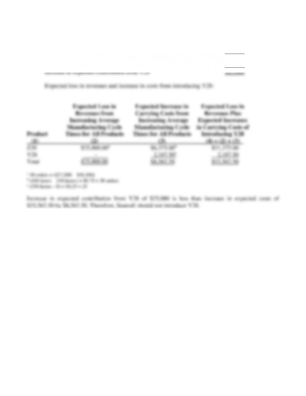
Y28 – 2,187.50c 2,187.50
Total $25,000.00 $8,562.50 $33,562.50
a 50 orders × ($27,000 – $26,500)
b (410 hours – 240 hours) × $0.75 × 50 orders
c (350 hours – 0) × $0.25 × 25
Expected total costs 892,562.50 759,000.00 133,562.50
Expected revenues minus
expected costs $ 632,437.50 $ 591,000.00 $ 41,437.50
a (50 × $26,500) + (25 × $8,000) b 50 × $27,000
c (50 × $15,000) + (25 × $5,000) d 50 × $15,000
19-28
2. Selling price per order of Y28, which has an average
manufacturing lead time of more than 320 hours $ 6,000
Variable cost per order 5,000
Additional contribution per order of Y28 $ 1,000
Multiply by expected number of orders × 25
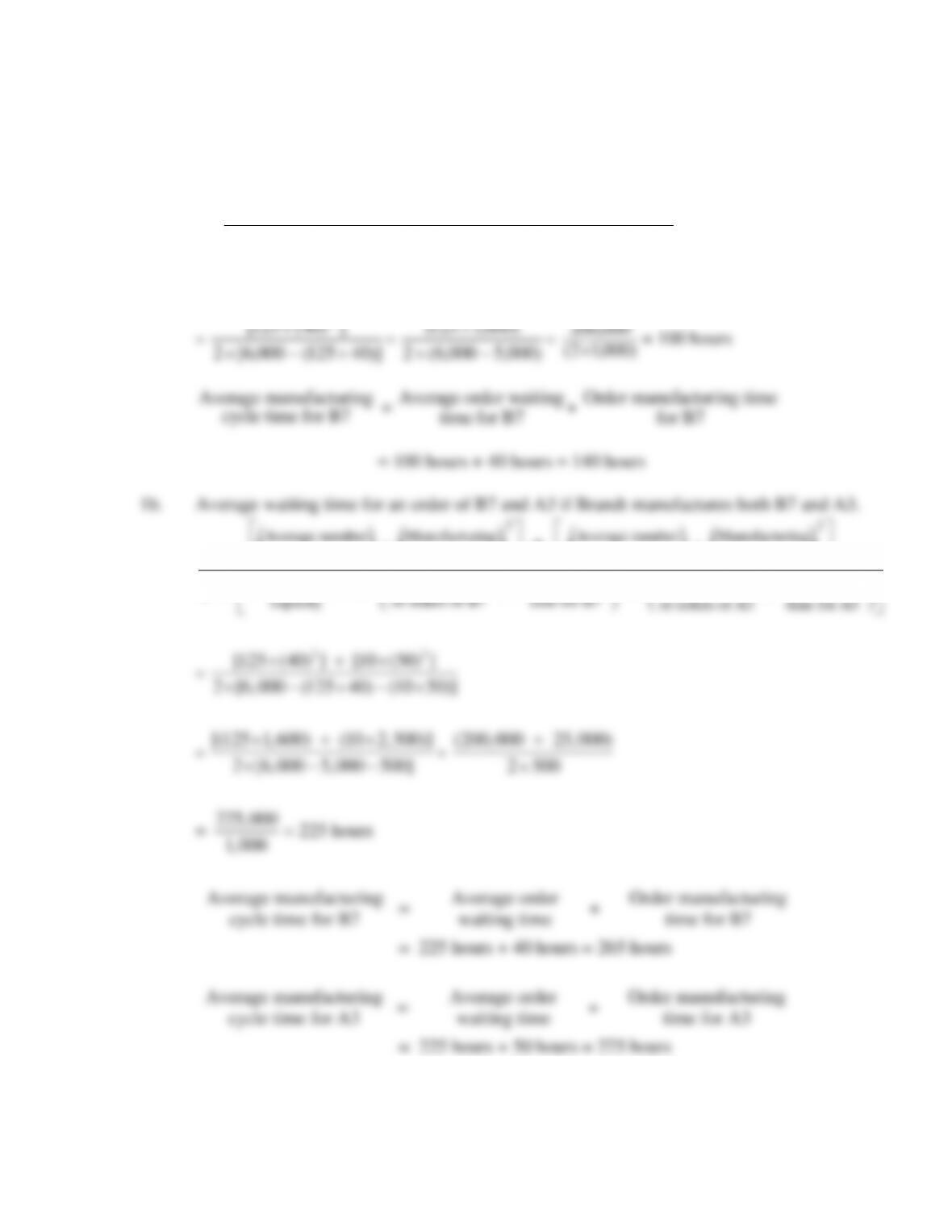
19-33 (40−45 min.) Manufacturing lead times, relevant revenues, and relevant costs.
1a. Average waiting time for an order of B7 if Brandt manufactures only B7
=
−
B7for time ingManufactur
B7 of orders of number Average
capacity
machine Annual
2
2
B7for time ingManufactur
B7 of orders of number Average
]
2
)40(125[
)600,1125(
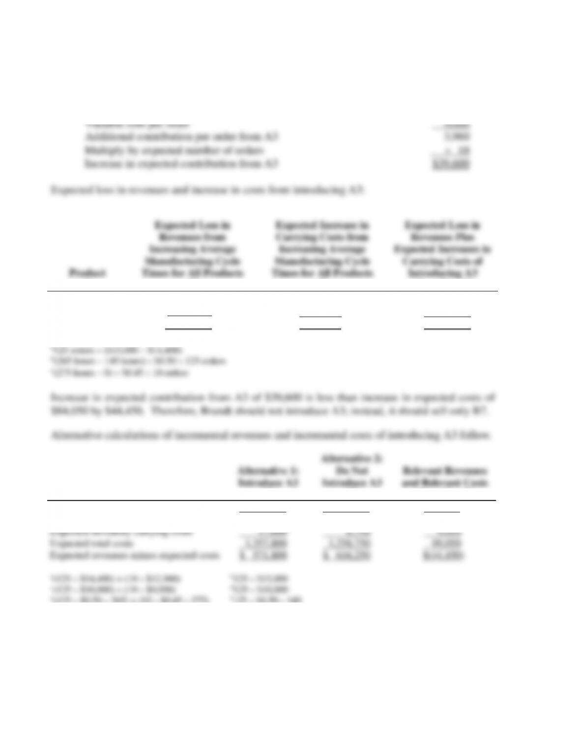
2. The direct approach is to look at incremental revenues and incremental costs of
manufacturing and selling A3.
Selling price per order for A3,
which has average operating throughput time of 275 hours $12,960