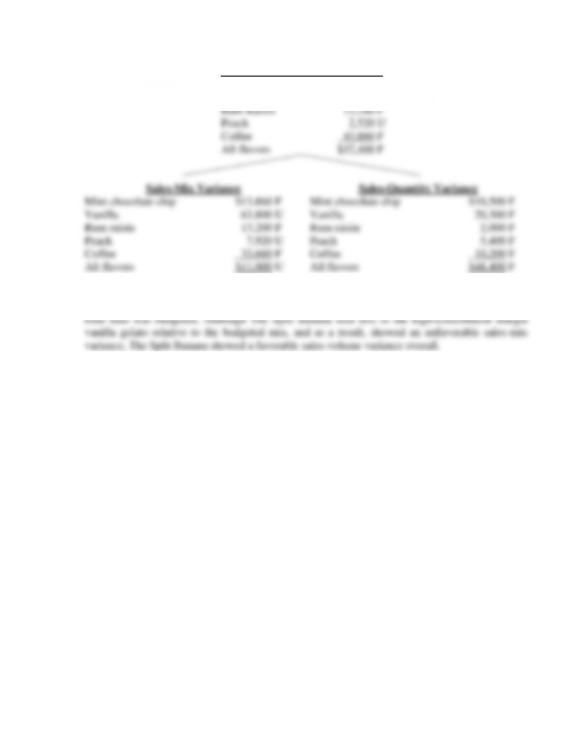
A summary of the variances is:
Sales-Volume Variance
Mint chocolate chip $24,360 F
Vanilla 43,500 U
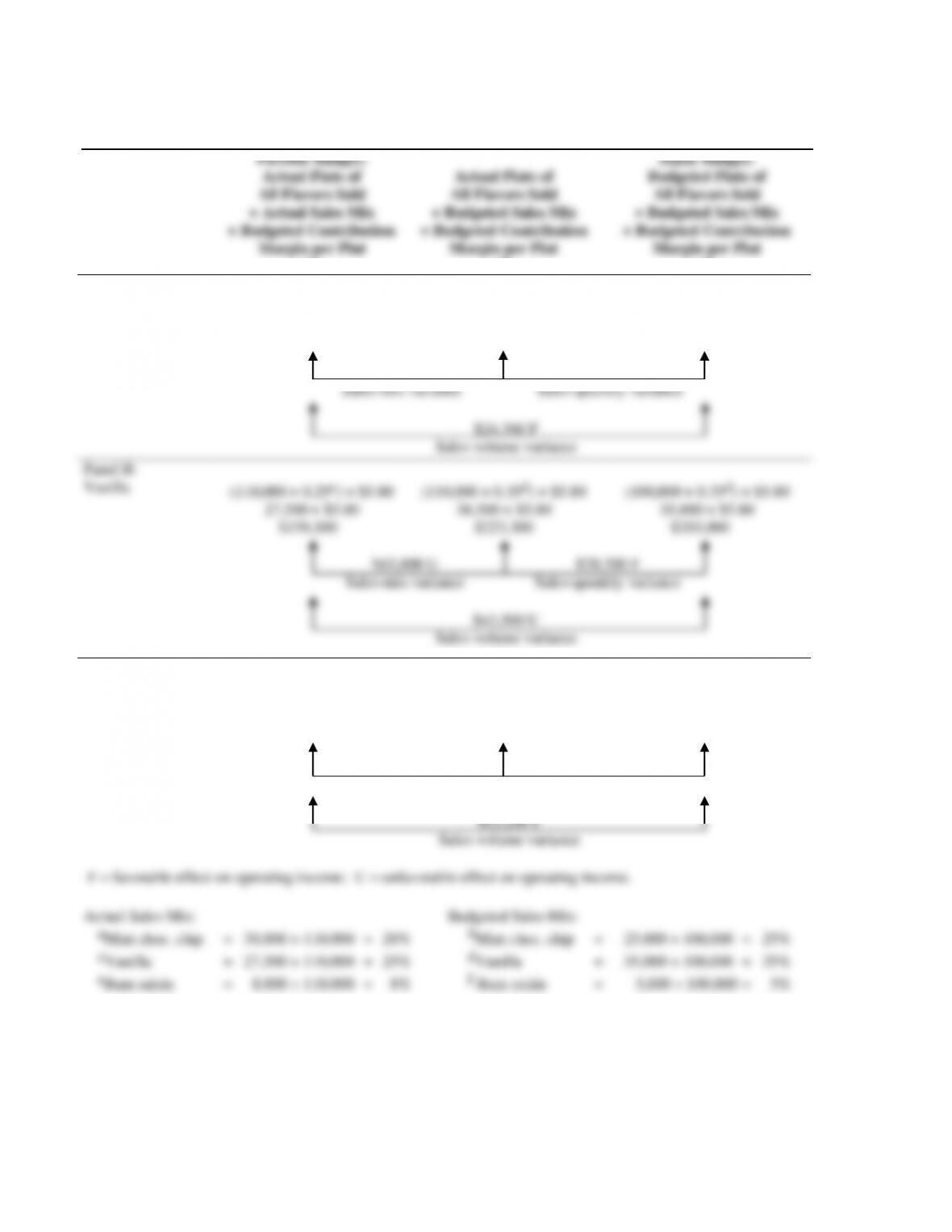
SOLUTION EXHIBIT 14-34
Columnar Presentation of Sales-Volume, Sales-Quantity, and Sales-Mix Variances
for The Split Banana
Flexible Budget:
Actual Pints of
All Flavors Sold
× Actual Sales Mix
× Budgeted Contribution
Margin per Pint
(1)
Actual Pints of
All Flavors Sold
× Budgeted Sales Mix
× Budgeted Contribution
Margin per Pint
(2)
Static Budget:
Budgeted Pints of
All Flavors Sold
× Budgeted Sales Mix
× Budgeted Contribution
Margin per Pint
(3)
Panel A:
Mint choc. chip
(110,000 × 0.28a) × $4.20
30,800 × $4.20
(110,000 × 0.25b) × $4.20
27,500 × $4.20
(100,000 × 0.25b) × $4.20
25,000 × $4.20
$129,360 $115,500 $105,000
Panel B:
Vanilla
(110,000 × 0.25c) × $5.80
27,500 × $5.80
(110,000 × 0.35d) × $5.80
38,500 × $5.80
(100,000 × 0.35d) × $5.80
35,000 × $5.80
$159,500 $223,300 $203,000
Panel C:
Rum Raisin
(110,000 × 0.08e) × $4.00
8,800 × $4.00
(110,000 × 0.05f) × $4.00
5,500 × $4.00
(100,000 × 0.05f) × $4.00
5,000 × $4.00
$35,200 $22,000 $20,000
$13,860 F
Sales-mix variance
$10,500 F
Sales-quantity variance
$24,360 F
Sales-volume variance
$63,800 U
Sales-mix variance
$20,300 F
Sales-quantity variance
$43,500 U
Sales-volume variance
$13,200 F
Sales-mix variance
$2,000 F
Sales-quantity variance
$15,200 F
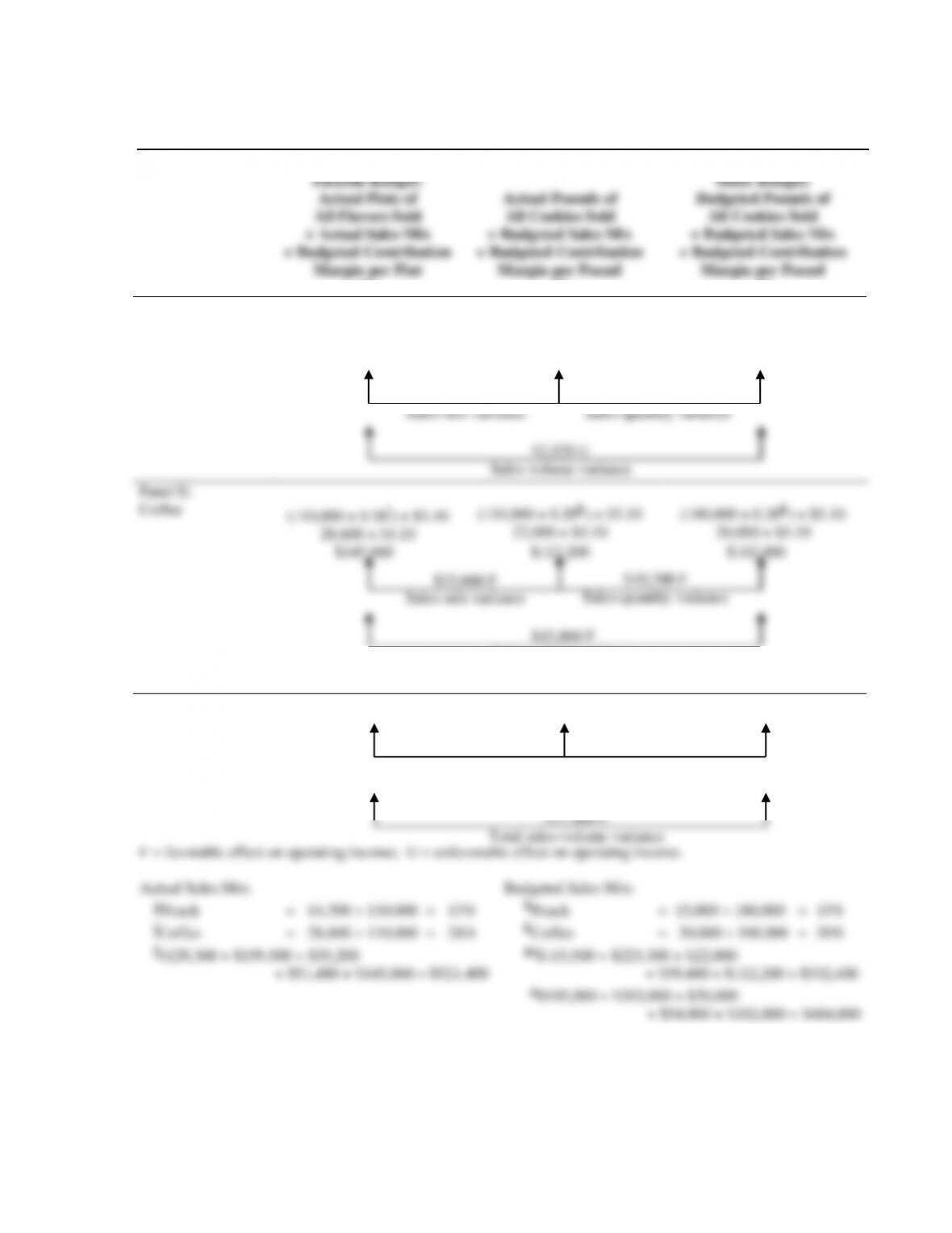
SOLUTION EXHIBIT 14-34 (Cont’d.)
Columnar Presentation of Sales-Volume, Sales-Quantity, and Sales-Mix Variances
for The Split Banana
Flexible Budget:
Actual Pints of
All Flavors Sold
× Actual Sales Mix
× Budgeted Contribution
Margin per Pint
(1)
Actual Pounds of
All Cookies Sold
× Budgeted Sales Mix
× Budgeted Contribution
Margin per Pound
(2)
Static Budget:
Budgeted Pounds of
All Cookies Sold
× Budgeted Sales Mix
× Budgeted Contribution
Margin per Pound
(3)
Panel D:
Peach
(110,000 × 0.13g) × $3.60
14,300 × $3.60
(110,000 × 0.15h) × $3.60
16,500 × $3.60
(100,000 × 0.15h) × $3.60
15,000 × $3.60
$51,480 $59,400 $54,000
Panel E:
Coffee
(110,000 × 0.26j) × $5.10
28,600 × $5.10
(110,000 × 0.20k) × $5.10
22,000 × $5.10
(100,000 × 0.20k) × $5.10
20,000 × $5.10
$145,860 $112,200 $102,000
Panel F: $521,400l $532,400m $484,000n
All Flavors
F = favorable effect on operating income; U = unfavorable effect on operating income.
Actual Sales Mix:
gPeach = 14,300 ÷ 110,000 = 13%
jCoffee = 28,600 ÷ 110,000 = 26%
l$129,360 + $159,500 + $35,200
+ $51,480 + $145,860 = $521,400
Budgeted Sales Mix:
hPeach = 15,000 ÷ 100,000 = 15%
kCoffee = 20,000 ÷ 100,000 = 20%
m$115,500 + $223,300 + $22,000
+ $59,400 + $112,200 = $532,400
n$105,000 + $203,000 + $20,000
+ $54,000 + $102,000 = $484,000
$7,920 U
Sales-mix variance
$5,400 F
Sales-quantity variance
$2,520 U
Sales-volume variance
$33,660 F
Sales-mix variance
$10,200 F
Sales-quantity variance
$43,860 F
Sales-volume variance
$11,000 U
Total sales-mix variance
$48,400 F
Total sales-quantity variance
$37,400 F
Total sales-volume variance
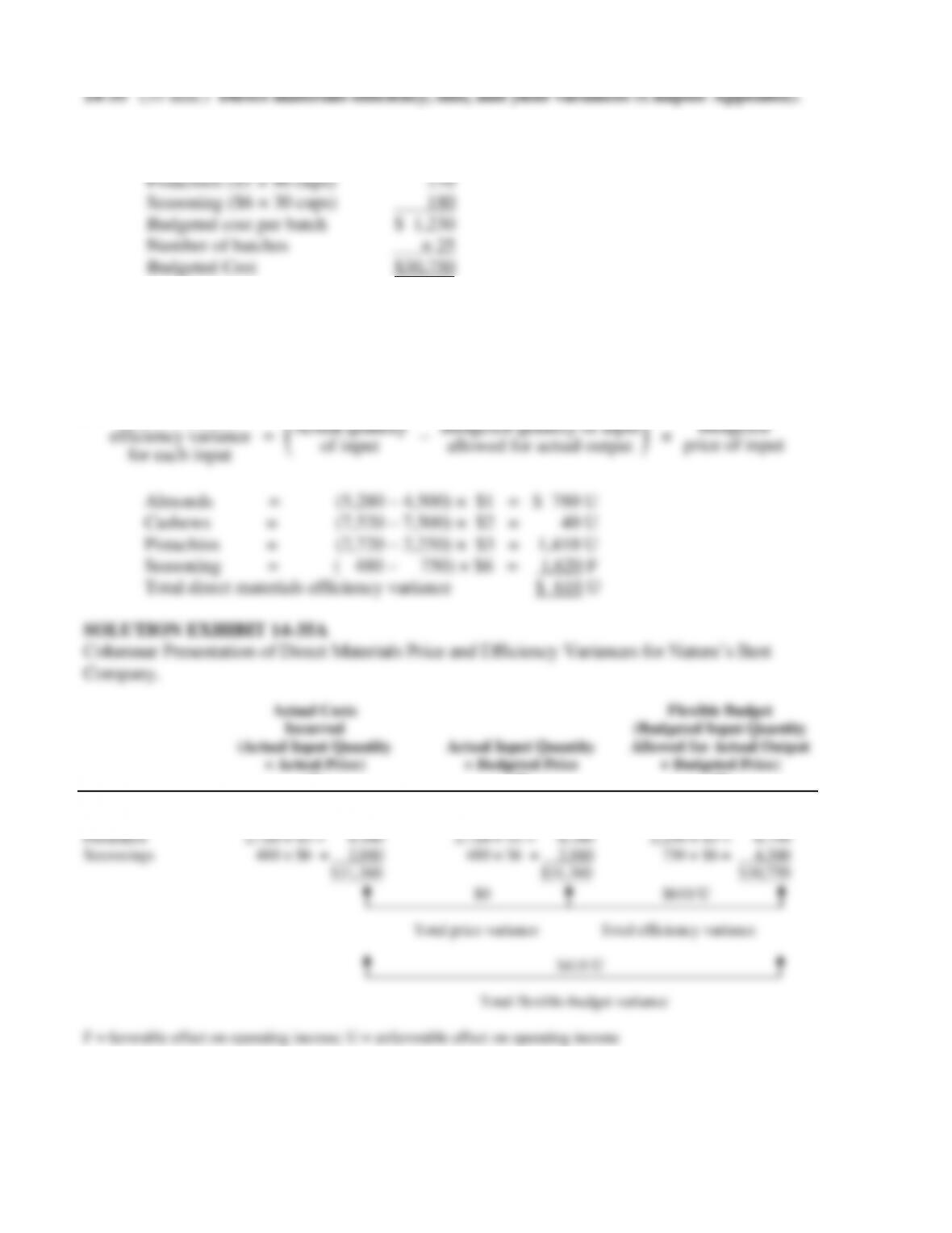
1. Almonds ($1 × 180 cups) $ 180
Cashews ($2 × 300 cups) 600
2. Solution Exhibit 14-35A presents the total price variance ($0), the total efficiency
variance ($610 U), and the total flexible-budget variance ($610 U).
Total direct materials efficiency variance can also be computed as:
Direct materials
efficiency variance
for each input
=
( )
Actual quantity Budgeted quantity of input
of input allowed for actual output
−
×
Budgeted
price of input
Almonds = (5,280 – 4,500) × $1 = $ 780 U
Cashews = (7,520 – 7,500) × $2 = 40 U
Pistachios = (2,720 – 2,250) × $3 = 1,410 U
Seasoning = ( 480 – 750) × $6 = 1,620 F
Total direct materials efficiency variance $ 610 U
SOLUTION EXHIBIT 14-35A
Columnar Presentation of Direct Materials Price and Efficiency Variances for Nature’s Best
Company.
Actual Costs
Incurred
(Actual Input Quantity
× Actual Price)
(1)
Actual Input Quantity
× Budgeted Price
(2)
Flexible Budget
(Budgeted Input Quantity
Allowed for Actual Output
× Budgeted Price)
(3)
Almonds
5,280 × $1 = $ 5,280
5,280 × $1 = $ 5,280
4,500 × $1 = $ 4,500
Cashews
7,520 × $2 = 15,040
7,520 × $2 = 15,040
7,500 × $2 = 15,000
Pistachios
2,720 × $3 = 8,160
2,720 × $3 = 8,160
2,250 × $3 = 6,750
Seasonings
480 × $6 = 2,880
480 × $6 = 2,880
750 × $6 = 4,500
$31,360
$31,360
$30,750
$0 $610 U
Total price variance Total efficiency variance
$610 U
Total flexible-budget variance
F = favorable effect on operating income; U = unfavorable effect on operating income
14-45
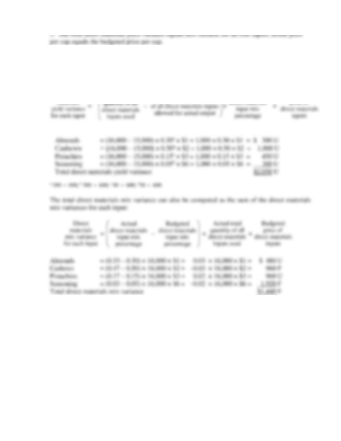
4. Solution Exhibit 14-35B presents the total direct materials yield and mix variances.
The total direct materials yield variance can also be computed as the sum of the direct
materials yield variances for each input:
Direct
materials
yield variance
for each input
=
Actual total Budgeted total quantity
quantity of all of all direct materials inputs
direct materials allowed for actual output
inputs used
−
×
Budgeted
direct materials
input mix
percentage
×
Budgeted
price of
direct materials
inputs
Almonds = (16,000 – 15,000) × 0.30a × $1 = 1,000 × 0.30 × $1 = $ 300 U
Cashews = (16,000 – 15,000) × 0.50b × $2 = 1,000 × 0.50 × $2 = 1,000 U
Pistachios = (16,000 – 15,000) × 0.15c × $3 = 1,000 × 0.15 × $3 = 450 U
Seasoning = (16,000 – 15,000) × 0.05d × $6 = 1,000 × 0.05 × $6 = 300 U
Total direct materials yield variance $2,050 U
a 180
600; b 300
600; c 90
600; d30
600
The total direct materials mix variance can also be computed as the sum of the direct materials
mix variances for each input:
Direct
materials
mix variance
for each input
=
Actual Budgeted
direct materials direct materials
input mix input mix
percentage percentage
−
×
Actual total
quantity of all
direct materials
inputs used
×
Budgeted
price of
direct materials
inputs
Almonds = (0.33 – 0.30) × 16,000 × $1 = 0.03 × 16,000 × $1 = $ 480 U
Cashews = (0.47 – 0.50) × 16,000 × $2 = –0.03 × 16,000 × $2 = 960 F
Pistachios = (0.17 – 0.15) × 16,000 × $3 = 0.02 × 16,000 × $3 = 960 U
Seasoning = (0.03 – 0.05) × 16,000 × $6 = –0.02 × 16,000 × $6 = 1,920 F
Total direct materials mix variance $1,440 F
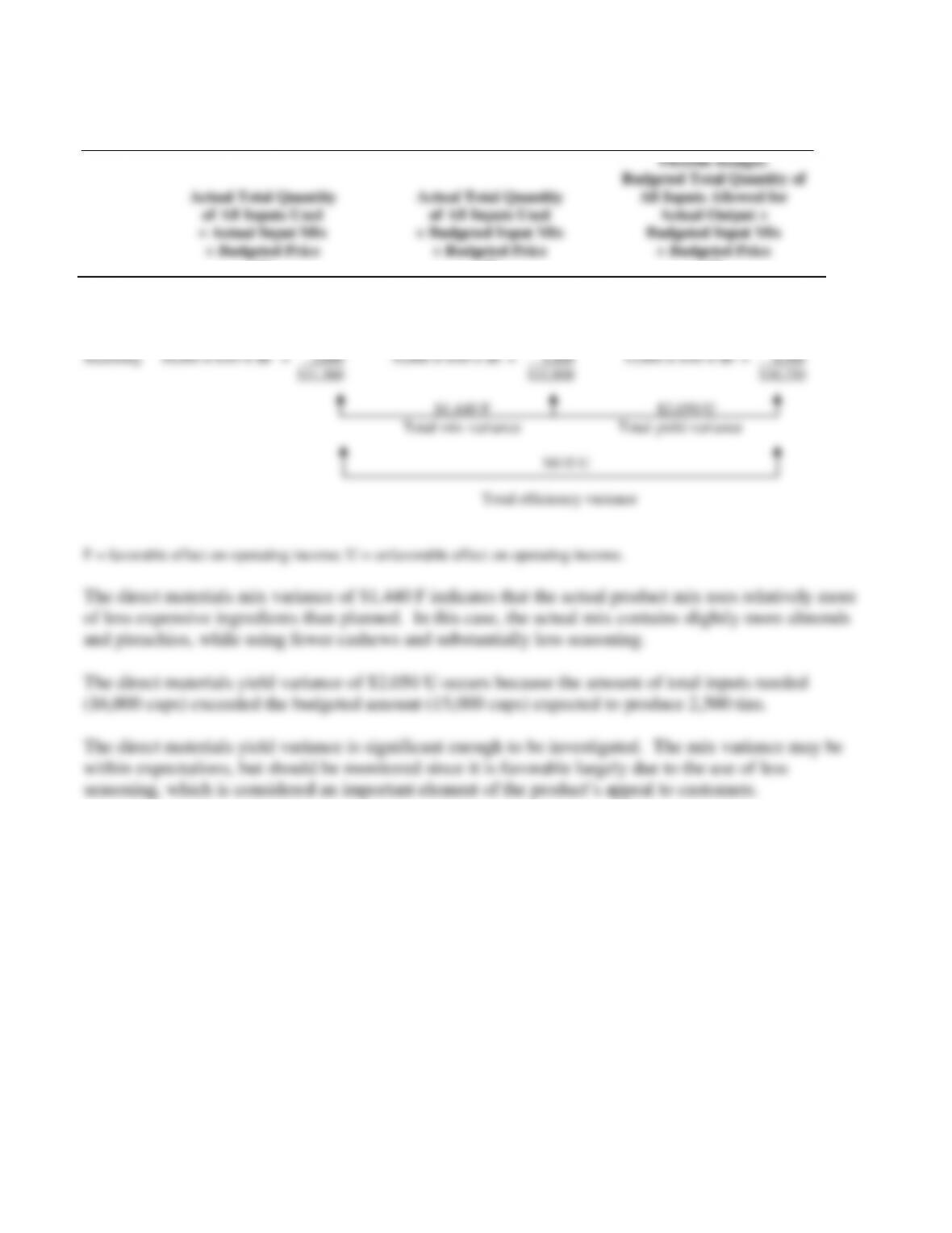
SOLUTION EXHIBIT 14-35B
Columnar Presentation of Direct Materials Yield and Mix Variances for Nature’s Best Company.
Actual Total Quantity
of All Inputs Used
× Actual Input Mix
× Budgeted Price
(1)
Actual Total Quantity
of All Inputs Used
× Budgeted Input Mix
× Budgeted Price
(2)
Flexible Budget:
Budgeted Total Quantity of
All Inputs Allowed for
Actual Output ×
Budgeted Input Mix
× Budgeted Price
(3)
Almonds 16,000 × 0.33 × $1 = $ 5,280
Cashews 16,000 × 0.47 × $2 = 15,040
Pistachios 16,000 × 0.17 × $3 = 8,160
Seasoning 16,000 × 0.03 × $6 = 2,880
$31,360
16,000 × 0.30 × $1 = $ 4,800
16,000 × 0.50 × $2 = 16,000
16,000 × 0.15 × $3 = 7,200
16,000 × 0.05 × $6 = 4,800
$32,800
15,000 × 0.30 × $1 = $ 4,500
15,000 × 0.50 × $2 = 15,000
15,000 × 0.15 × $3 = 6,750
15,000 × 0.05 × $6 = 4,500
$30,750
$1,440 F $2,050 U
Total mix variance Total yield variance
$610 U
Total efficiency variance
F = favorable effect on operating income; U = unfavorable effect on operating income.
The direct materials mix variance of $1,440 F indicates that the actual product mix uses relatively more
of less expensive ingredients than planned. In this case, the actual mix contains slightly more almonds
and pistachios, while using fewer cashews and substantially less seasoning.
The direct materials yield variance of $2,050 U occurs because the amount of total inputs needed
(16,000 cups) exceeded the budgeted amount (15,000 cups) expected to produce 2,500 tins.
The direct materials yield variance is significant enough to be investigated. The mix variance may be
within expectations, but should be monitored since it is favorable largely due to the use of less
seasoning, which is considered an important element of the product’s appeal to customers.
14-47
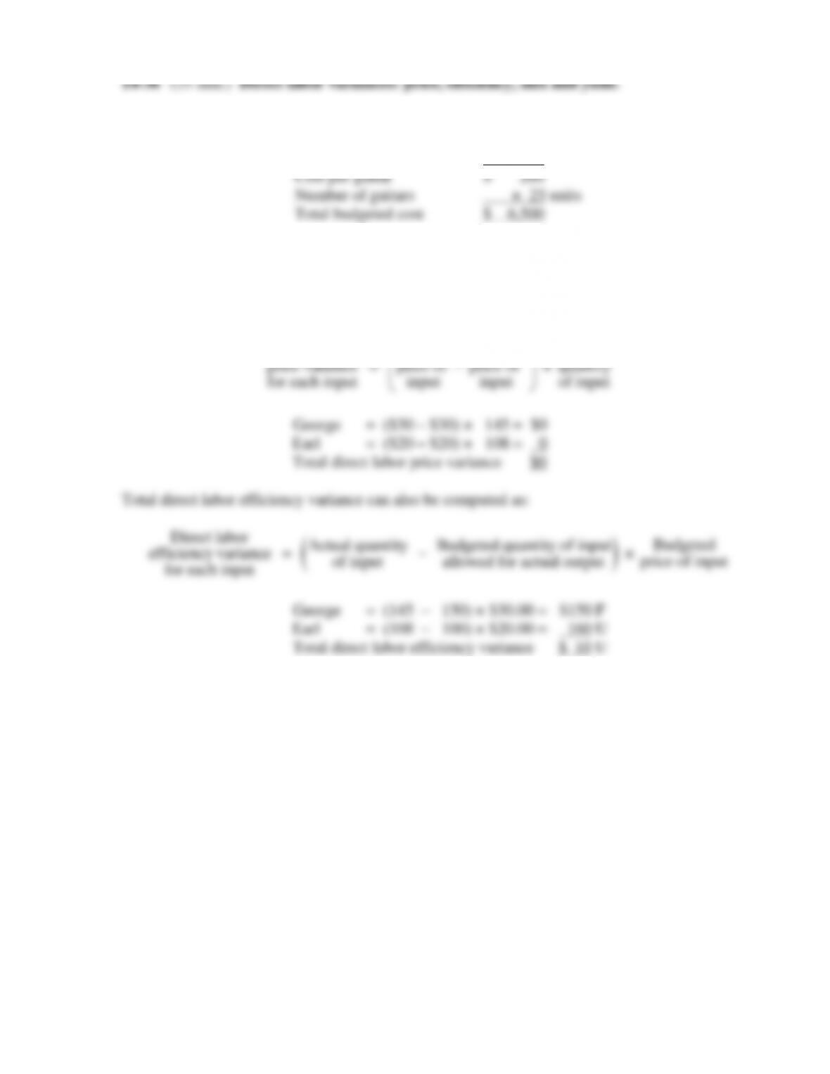
1.
George ($30 × 6 hrs.)
$ 180
Earl ($20 × 4 hrs.)
80
Cost per guitar
$ 260
Number of guitars
× 25 units
Total budgeted cost
$ 6,500
2. Solution Exhibit 14-36A presents the total price variance ($0), the total efficiency variance
($10 U), and the total flexible-budget variance ($10U).
Total direct labor price variance can also be computed as:
Direct labor
price variance
for each input
=
Actual Budgeted
price of price of
input input
−
×
Actual
quantity
of input
George = ($30 – $30) × 145 = $0
Earl = ($20 – $20) × 108 = 0
Total direct labor price variance $0
Total direct labor efficiency variance can also be computed as:
Direct labor
efficiency variance
for each input
=
( )
Actual quantity Budgeted quantity of input
of input allowed for actual output
−
×
Budgeted
price of input
George = (145 – 150) × $30.00 = $150 F
Earl = (108 – 100) × $20.00 = 160 U
Total direct labor efficiency variance $ 10 U
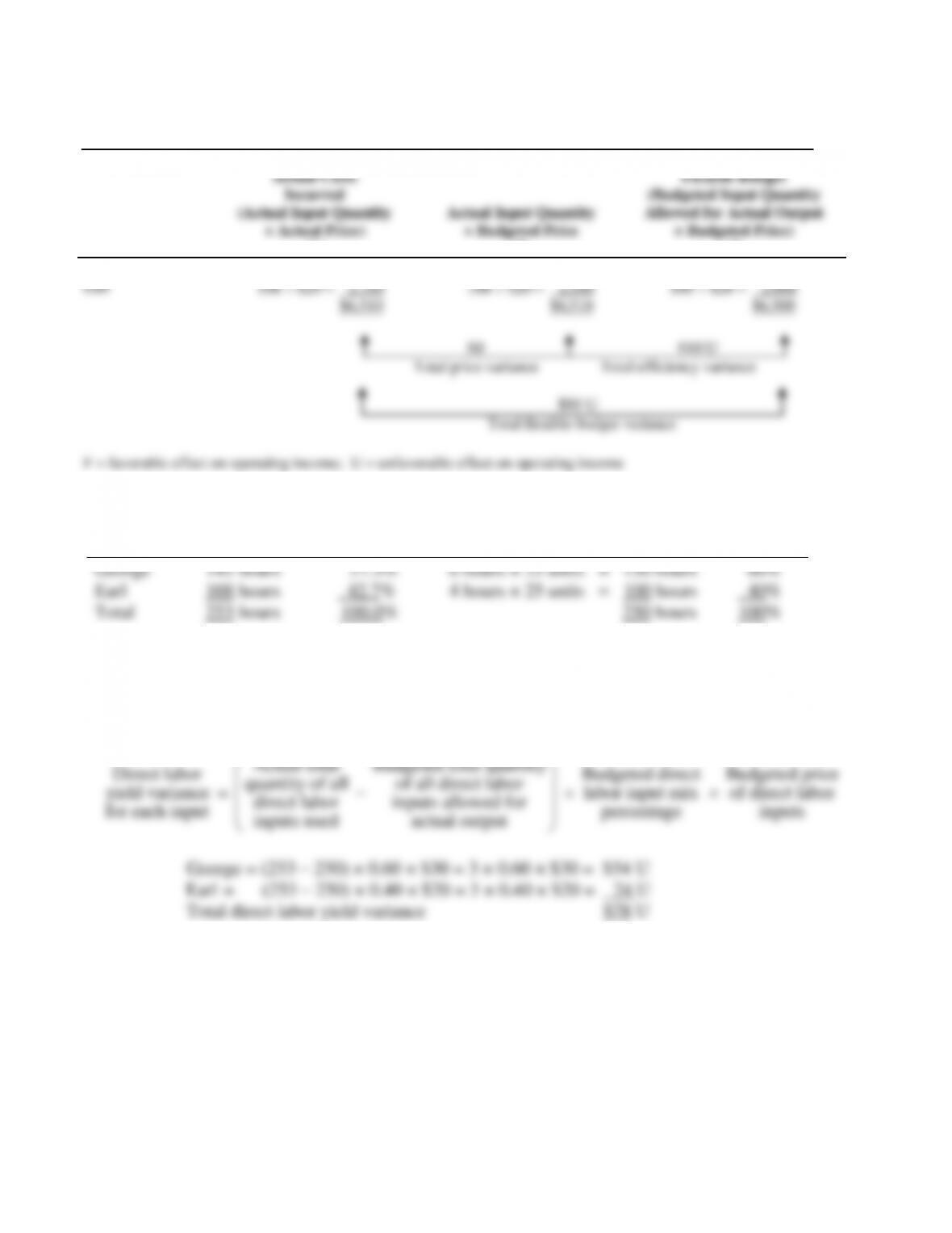
SOLUTION EXHIBIT 14-36A
Columnar Presentation of Direct Labor Price and Efficiency Variances for Trevor Joseph Guitars
Actual Costs
Incurred
(Actual Input Quantity
× Actual Price)
(1)
Actual Input Quantity
× Budgeted Price
(2)
Flexible Budget
(Budgeted Input Quantity
Allowed for Actual Output
× Budgeted Price)
(3)
George
145 $30 = $4,350
145 $30 = $4,350
150 $30 = $4,500
Earl
108 $20 = 2,160
108 $20 = 2,160
100 $20 = 2,000
$6,510
$6,510
$6,500
$0 $10 U
Total price variance Total efficiency variance
$10 U
Total flexible-budget variance
F = favorable effect on operating income; U = unfavorable effect on operating income
3.
Actual Quantity
of Input
Actual
Mix
Budgeted Quantity
of Input for Actual Output
Budgeted
Mix
George
145 hours
57.3%
6 hours × 25 units = 150 hours
60%
Earl
108 hours
42.7%
4 hours × 25 units = 100 hours
40%
Total
253 hours
100.0%
250 hours
100%
4. Solution Exhibit 14-36B presents the total direct labor yield and mix variances for Trevor
Joseph Guitars.
The total direct labor yield variance can also be computed as the sum of the direct labor
yield variances for each input:
Direct labor
Actual total
quantity of all
Budgeted total quantity
of all direct labor
Budgeted direct
Budgeted price