10-38
10-40 (40–50 min.) Purchasing Department cost drivers, activity-based costing, simple
regression analysis.
2. Both Regressions 2 and 3 are well-specified regression models. The slope coefficients on
their respective independent variables are significantly different from zero. These results support
the Couture Fabrics’ presentation in which the number of purchase orders and the number of
3. Guidelines presented in the chapter could be used to gain additional evidence on cost
drivers of purchasing department costs.
1. Use physical relationships or engineering relationships to establish cause-and-effect
10-39
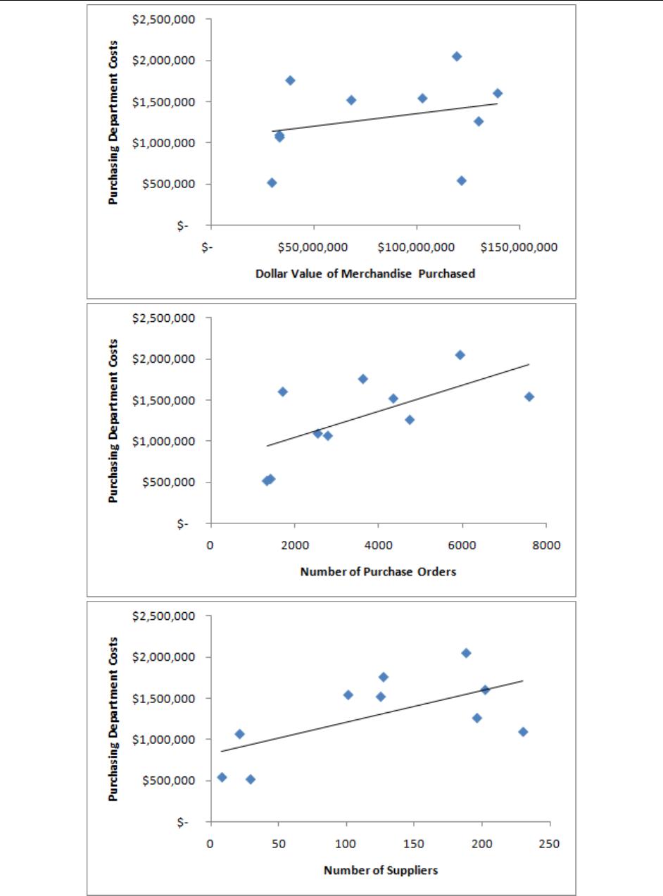
SOLUTION EXHIBIT 10-40A
Regression Lines of Various Cost Drivers for Purchasing Dept. Costs for Fashion Bling
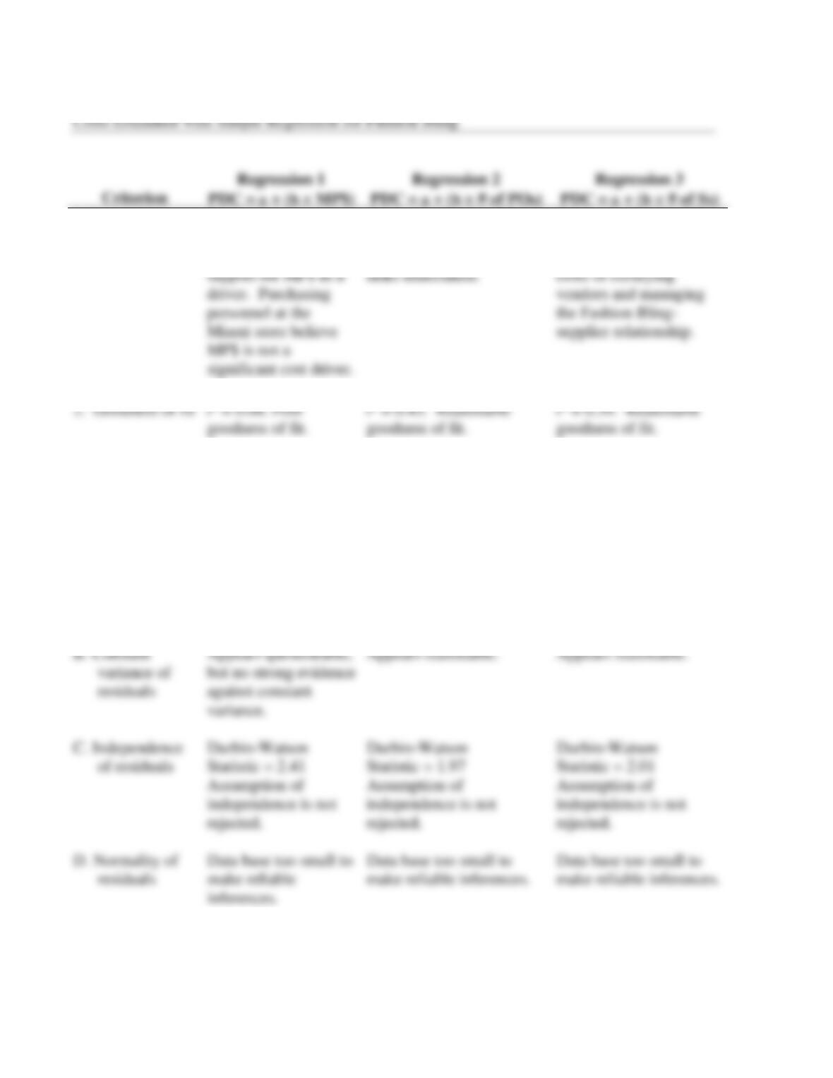
SOLUTION EXHIBIT 10-40B
Comparison of Alternative Cost Functions for Purchasing Department
10-41
10-41 (30–40 min.) Purchasing Department cost drivers, multiple regression analysis
(continuation of 10-40) (chapter appendix).
1. Regression 4 is a well-specified regression model:
Economic plausibility: Both independent variables are plausible and are supported by the
findings of the Couture Fabrics study.
Goodness of fit: The r2 of 0.64 indicates an excellent goodness of fit.
2. Regression 5 adds an additional independent variable (MP$) to the two independent
variables in Regression 4. This additional variable (MP$) has a t-value of 0.01, implying its slope
3. Budgeted purchasing department costs for the Baltimore store next year are
$484,522 + ($126.66 4,000) + ($2,903 95) = $1,266,947
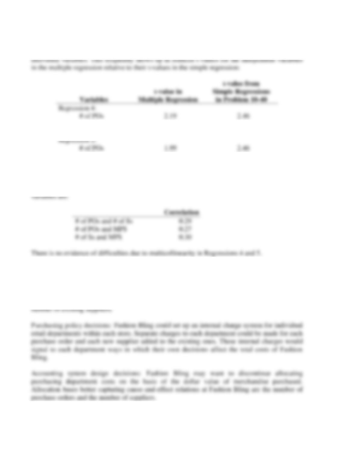
4. Multicollinearity is a frequently encountered problem in cost accounting; it does not arise
in simple regression because there is only one independent variable in a simple regression. One
consequence of multicollinearity is an increase in the standard errors of the coefficients of the
10-42 (25 min.) Interpreting regression results, matching time periods, ethics
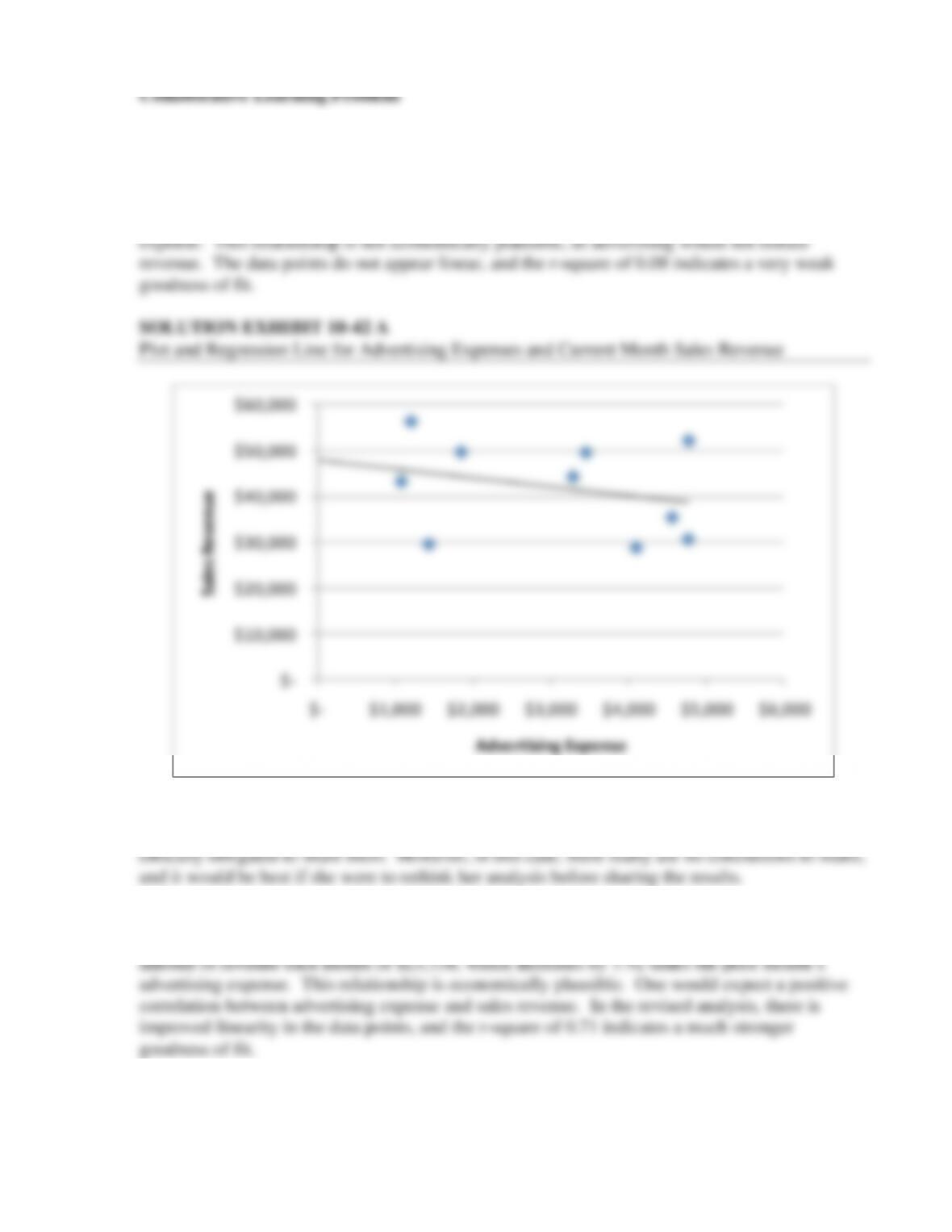
1. SOLUTION EXHIBIT 10-42A presents the data plot for the initial analysis. The formula
of Revenue = $47,801 – (1.92 × Advertising expense) indicates that there is a fixed amount of
revenue each month of $47,801, which is reduced by 1.92 times that month’s advertising
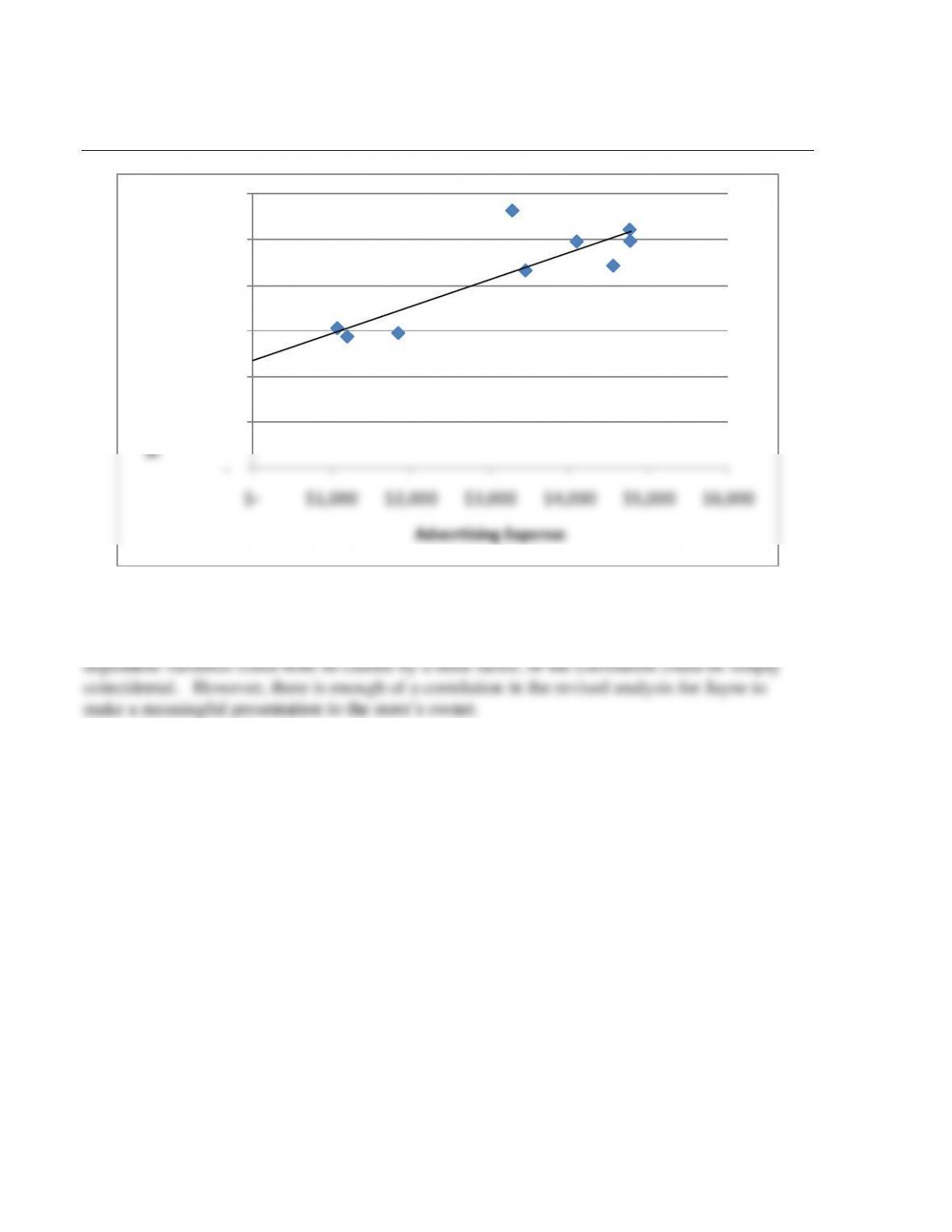
SOLUTION EXHIBIT 10-42B
Plot and Regression Line for Advertising Expense and Following Month Sales Revenue
–
10,000
20,000
30,000
40,000
50,000
60,000
$– $1,000 $2,000 $3,000 $4,000 $5,000 $6,000
Sales Revenue (Following Month)
Advertising Expense
4. Jayne must be very careful about making conclusions regarding cause and effect. Even a
strong goodness of fit does not prove a cause and effect relationship. The independent and