10-37 (20–30 min.) Cost estimation, incremental unit-time learning model.
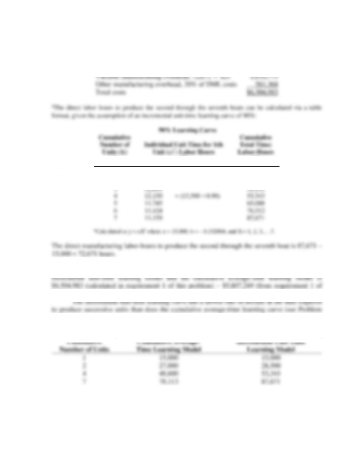
1. Cost to produce the 2nd through the 7th boats:
Direct materials, 6
$200,000
$1,200,000
Direct manufacturing labor (DML), 72,6711
$40
2,906,840
Variable manufacturing overhead, 72,671
$25
1,816,775
Other manufacturing overhead, 20% of DML costs
581,368
Total costs
$6,504,983
10-32
The reason is that, in the incremental unit-time learning model, as the number of units
double, only the last unit produced has a cost of 90% of the initial cost. In the cumulative
10-38 Regression; choosing among models. (chapter appendix)
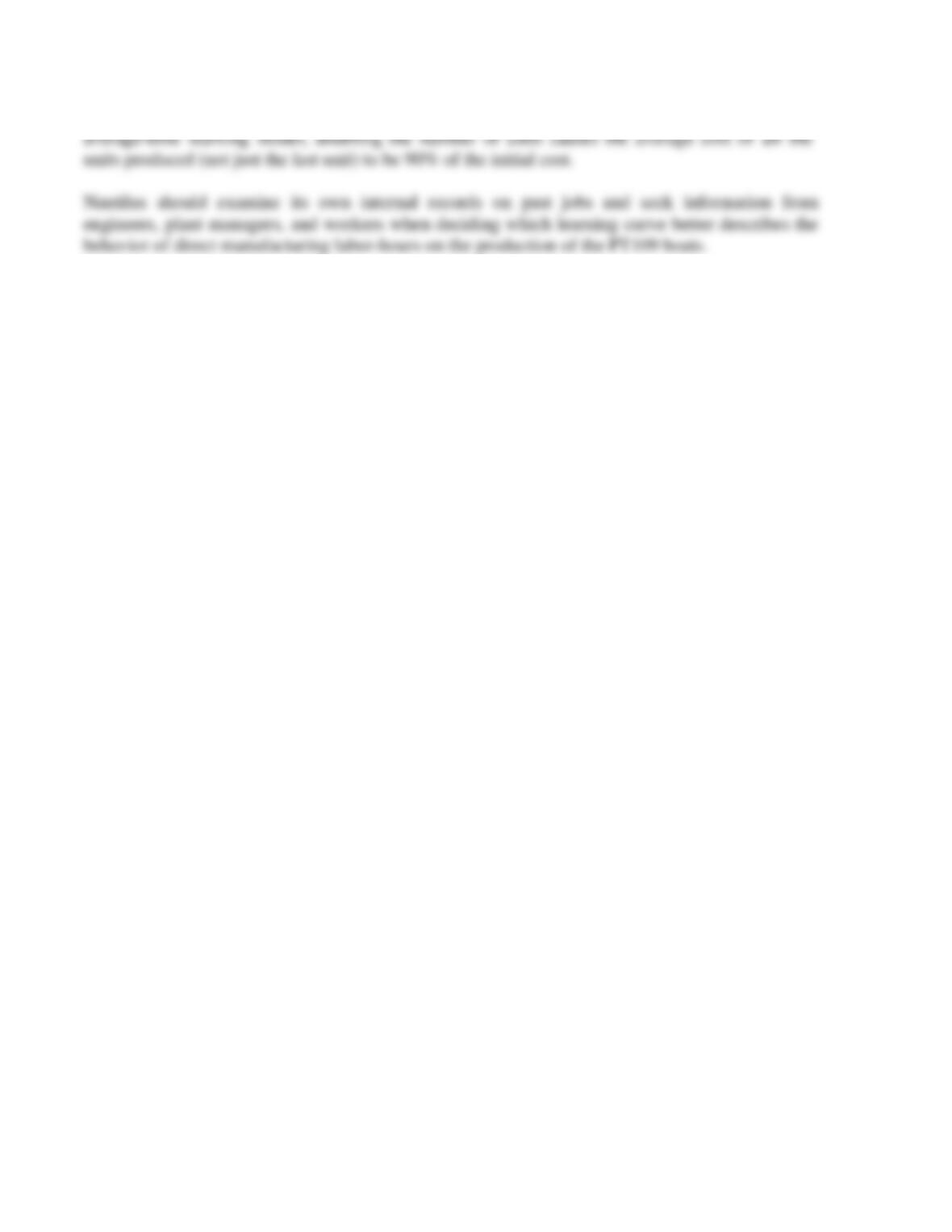
1. Solution Exhibit 10-38A presents the regression output for (a) setup costs and number of setups
and (b) setup costs and number of setup-hours.
SOLUTION EXHIBIT 10-38A
Regression Output for (a) Setup Costs and Number of Setups and (b) Setup Costs and Number of
Setup-Hours
a.
SUMMARY OUTPUT
Regression Statistics
Multiple R 0.686023489
R Square 0.470628228
Adjusted R Square 0.395003689
Standard Error 51385.93104
Observations 9
ANOVA
df SS MS F Significance F
Regression 1 16432501924 16432501924 6.223221 0.04131511
Residual 7 18483597365 2640513909
Total 8 34916099289
Coefficients Standard Error t Stat P-value Lower 95% Upper 95% Lower 95.0% Upper 95.0%
Intercept 12889.92611 61364.96556 0.210053505 0.839609 -132215.1596 157995.0118 -132215.1596 157995.0118
X Variable 1 426.7711823 171.0753629 2.494638474 0.041315 22.24223047 831.3001341 22.24223047 831.3001341
b.
SUMMARY OUTPUT
Regression Statistics
Multiple R 0.92242169
R Square 0.850861774
Adjusted R Square 0.829556313
Standard Error 27274.59603
Observations 9
ANOVA
df SS MS F Significance F
Regression 1 29708774168 29708774168 39.93632322 0.000396651
10-34
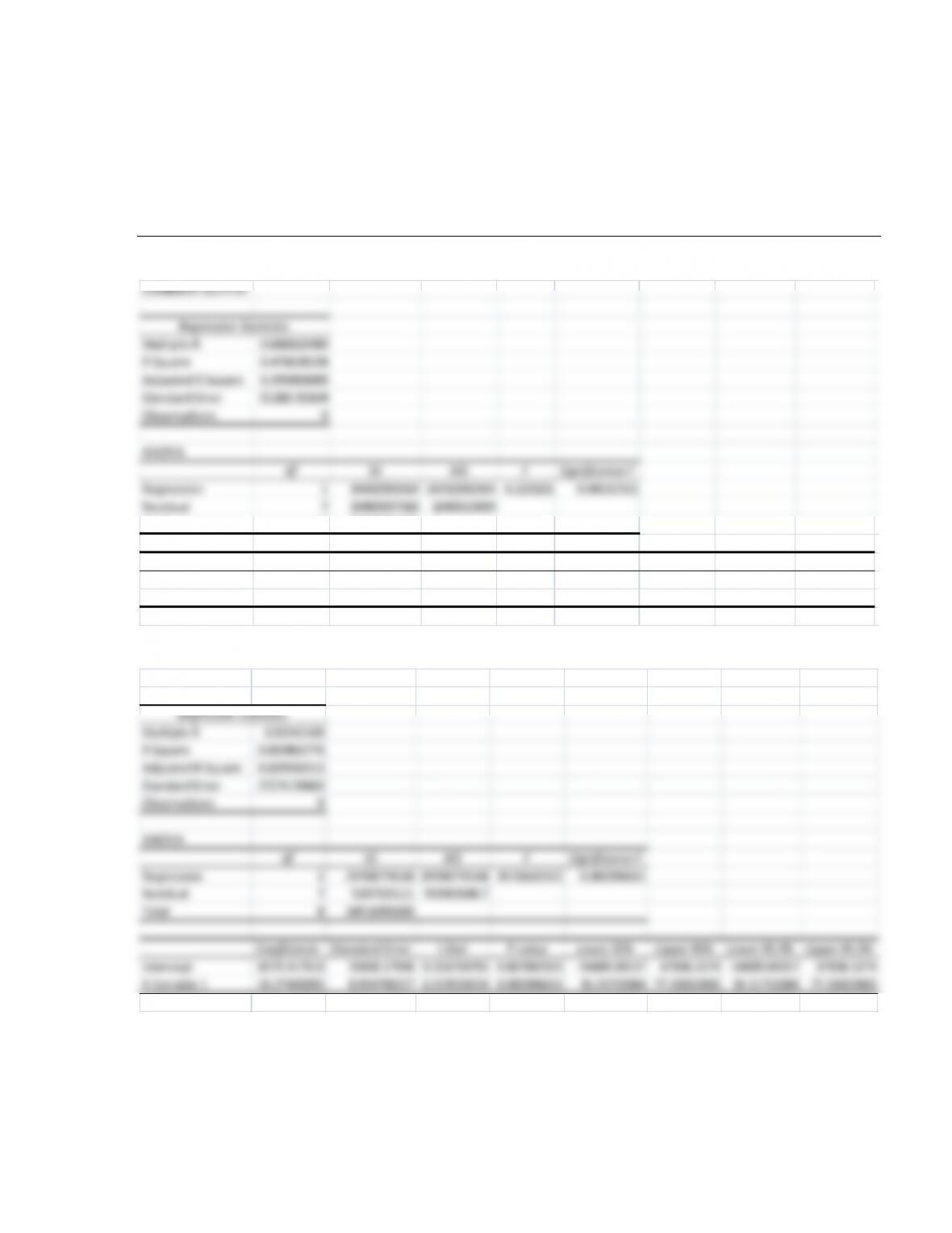
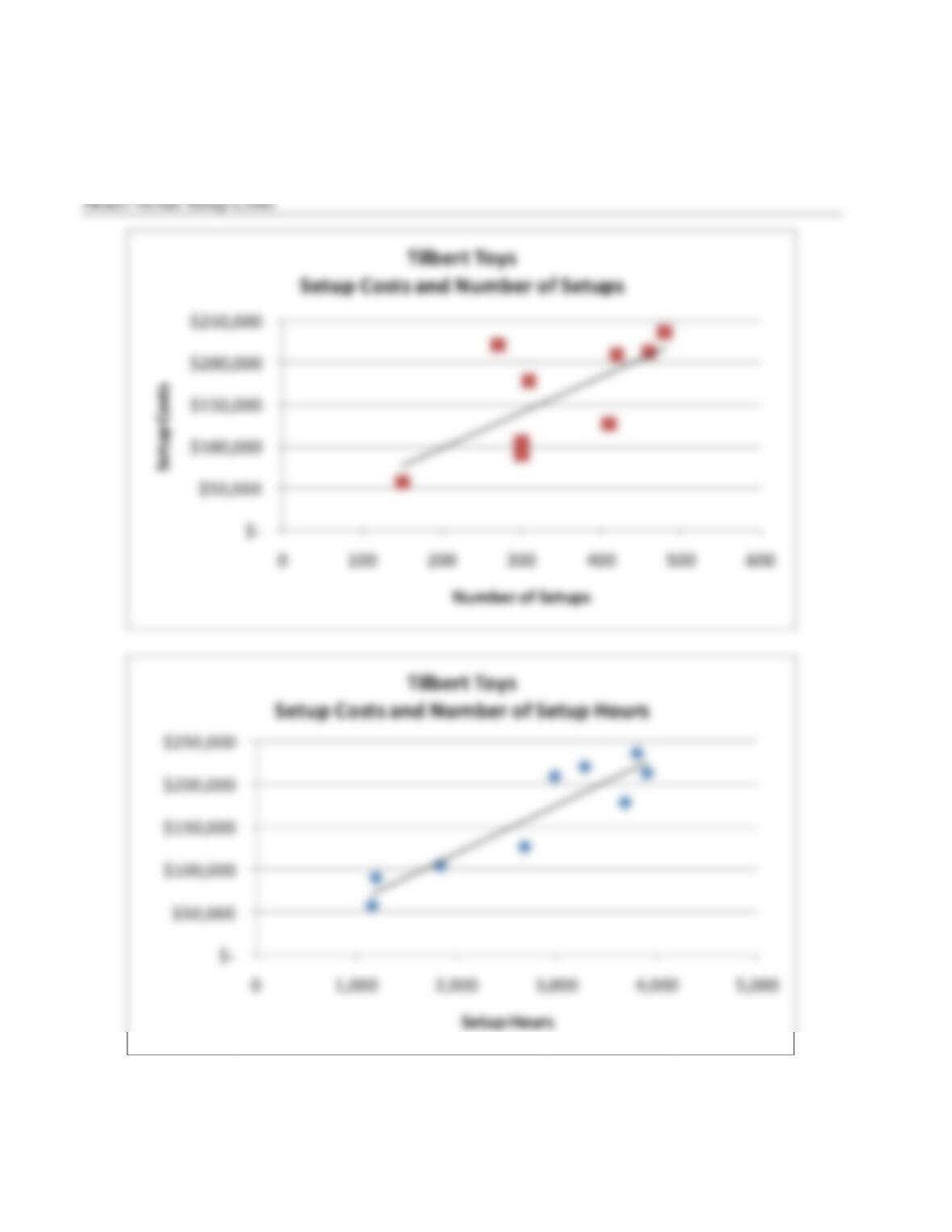
2. Solution Exhibit 10-38B presents the plots and regression lines for (a) number of setups versus
setup costs and (b) number of setup hours versus setup costs.
SOLUTION EXHIBIT 10-38B
Plots and Regression Lines for (a) Number of Setups versus Setup Costs and (b) Number of Setup–
3.
Number of Setups
Number of Setup Hours
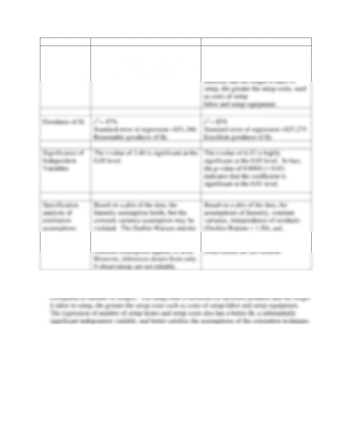
Economic
plausibility
A positive relationship
between setup costs
and the number of setups
is economically plausible.
A positive relationship between setup
costs and the number of setup-hours is
also economically plausible,
especially since setup time is not
uniform, and the longer it takes to
setup, the greater the setup costs, such
as costs of setup
labor and setup equipment.
Goodness of fit
r2 = 47%
Standard error of regression =$51,386
Reasonable goodness of fit.
r2 = 85%
Standard error of regression =$27,275
Excellent goodness of fit.
Significance of
Independent
Variables
The t-value of 2.49 is significant at the
0.05 level.
The t-value of 6.32 is highly
significant at the 0.05 level. In fact,
the p–value of 0.0004 (< 0.01)
indicates that the coefficient is
significant at the 0.01 level.
Specification
analysis of
estimation
assumptions
Based on a plot of the data, the
linearity assumption holds, but the
constant variance assumption may be
violated. The Durbin-Watson statistic
of 1.65 suggests the residuals are
independent. The normality of
residuals assumption appears to hold.
However, inferences drawn from only
9 observations are not reliable.
Based on a plot of the data, the
assumptions of linearity, constant
variance, independence of residuals
(Durbin-Watson = 1.50), and
normality of residuals hold. However,
inferences drawn from only 9
observations are not reliable.
4. The regression model using number of setup-hours should be used to estimate set up costs
because number of setup-hours is a more economically plausible cost driver of setup costs
10-39 (30min.) Multiple regression (continuation of 10-38).
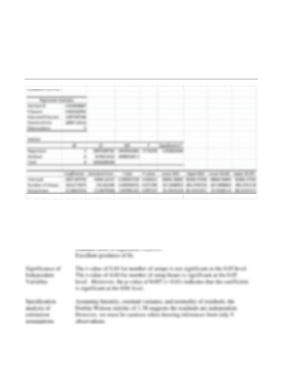
1. Solution Exhibit 10-39 presents the regression output for setup costs using both number of setups
and number of setup-hours as independent variables (cost drivers).
SOLUTION EXHIBIT 10-39
Regression Output for Multiple Regression for Setup Costs Using Both Number of Setups and
Number of Setup-Hours as Independent Variables (Cost Drivers)
SUMMARY OUTPUT
Regression Statistics
Multiple R 0.924938047
R Square 0.855510391
Adjusted R Square 0.807347188
Standard Error 28997.16516
Observations 9
ANOVA
df SS MS F Significance F
Regression 2 29871085766 14935542883 17.76274 0.003016545
Residual 6 5045013522 840835587.1
Total 8 34916099289
Coefficients Standard Error t Stat P-value Lower 95% Upper 95% Lower 95.0% Upper 95.0%
Intercept -2807.097769 34850.24247 –0.080547439 0.938421 –88082.56893 82468.37339 -88082.56893 82468.37339
Number of Setups 58.61773979 133.416589 0.439358705 0.675783 –267.8408923 385.0763718 –267.8408923 385.0763718
Setup Hours 52.30623518 13.08375044 3.997801352 0.007137 20.29145124 84.32101912 20.29145124 84.32101912
2.
Economic
plausibility
A positive relationship between setup costs and each of the independent
variables (number of setups and number of setup-hours) is economically
plausible.
Goodness of fit
r2 = 86%, Adjusted r2 = 81%
Standard error of regression =$28,997
Excellent goodness of fit.
Variables
estimation
assumptions
However, we must be cautious when drawing inferences from only 9
observations.
10-37
3. Multicollinearity is an issue that can arise with multiple regression but not simple regression
0.69 between number of setups and number of setup-hours. This is very close to the threshold of
0.70 that is usually taken as a sign of multicollinearity problems. As evidence, note the
4. The simple regression model using the number of setup-hours as the independent variable
achieves a comparable r2 to the multiple regression model. However, the multiple regression