10-21
Economic plausibility. The cost function shows a positive economically plausible relationship
between machine-hours and maintenance costs. There is a clear-cut engineering relationship of
3. Using the cost function estimated in 1, predicted maintenance costs would be $2 ×
100,000 = $200,000.
10-22
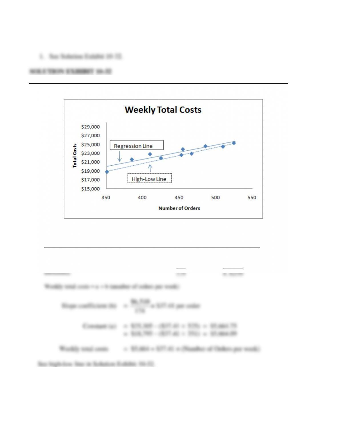
10-32 (30min.) High-low method and regression analysis.
2.
Number of
Orders per week
Weekly
Total Costs
Highest observation of cost driver (Week 9) 525 $25,305
Lowest observation of cost driver (Week 1) 351 18,795
10-23
Solution Exhibit 10-32 presents the regression line:
Weekly total costs = $8,631 + $31.92 × (Number of Orders per week)
Economic Plausibility. The cost function shows a positive economically plausible relationship
between number of orders per week and weekly total costs. Number of orders is a plausible cost
4. Profit =
Total weekly revenues + Total seasonal membership fees – Total weekly costs =
5. Let the average number of weekly orders be denoted by AWO. We want to find the
value of AWO for which Fresh Harvest will achieve zero profit. Using the format in
$80.8 × AWO = $41,310
10-24
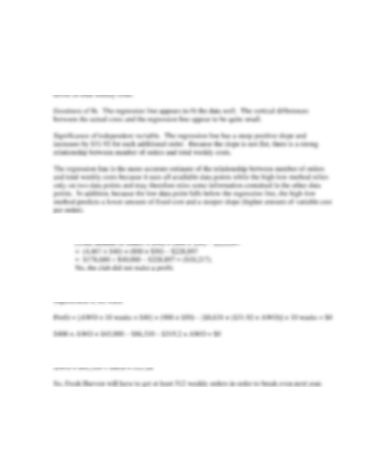
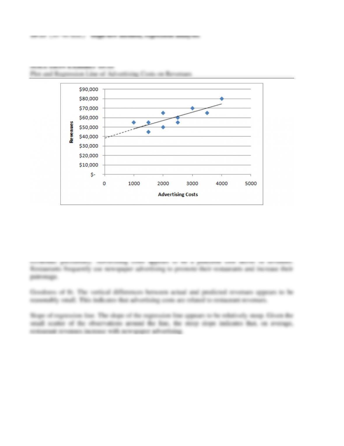
1. Solution Exhibit 10-33 presents the plots of advertising costs on revenues.
2. Solution Exhibit 10-33 also shows the regression line of advertising costs on revenues.
We evaluate the estimated regression equation using the criteria of economic plausibility,
goodness of fit, and slope of the regression line.
10-25
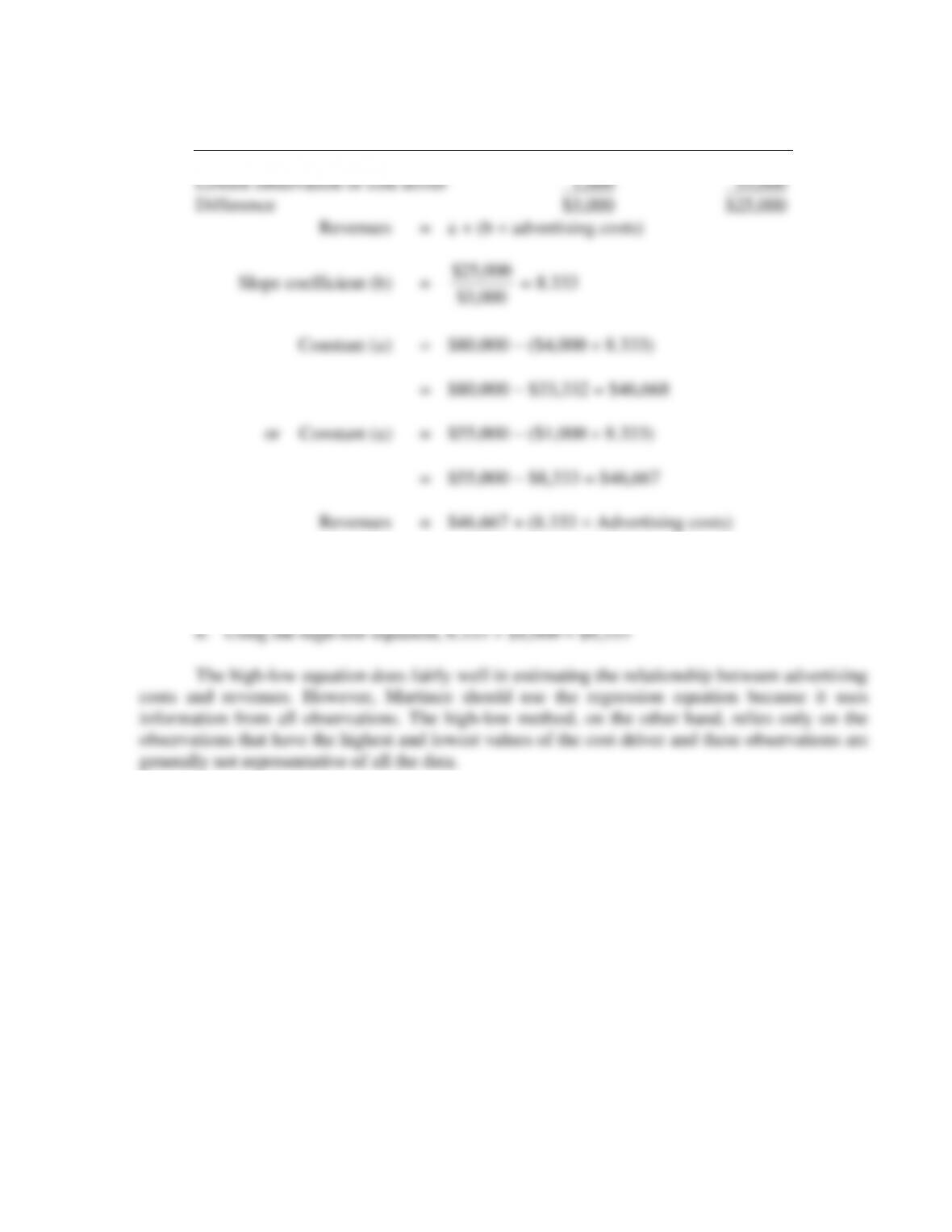
3. The high-low method would estimate the cost function as follows:
Advertising Costs Revenues
Highest observation of cost driver $4,000 $80,000
4. The increase in revenues for each $1,000 spent on advertising within the relevant range is
a. Using the regression equation, 8.723 $1,000 = $8,723
10-26
10-34 (30 min.) Regression, activity-based costing, choosing cost drivers.
1. Both number of units inspected and inspection labor-hours are plausible cost drivers for
inspection costs. The number of units inspected is likely related to test-kit usage, which is a
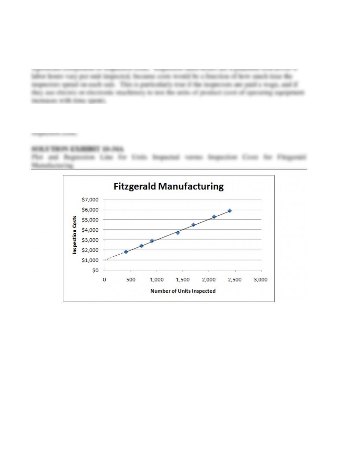
2. Solution Exhibit 10-34 presents (a) the plots and regression line for number of units inspected
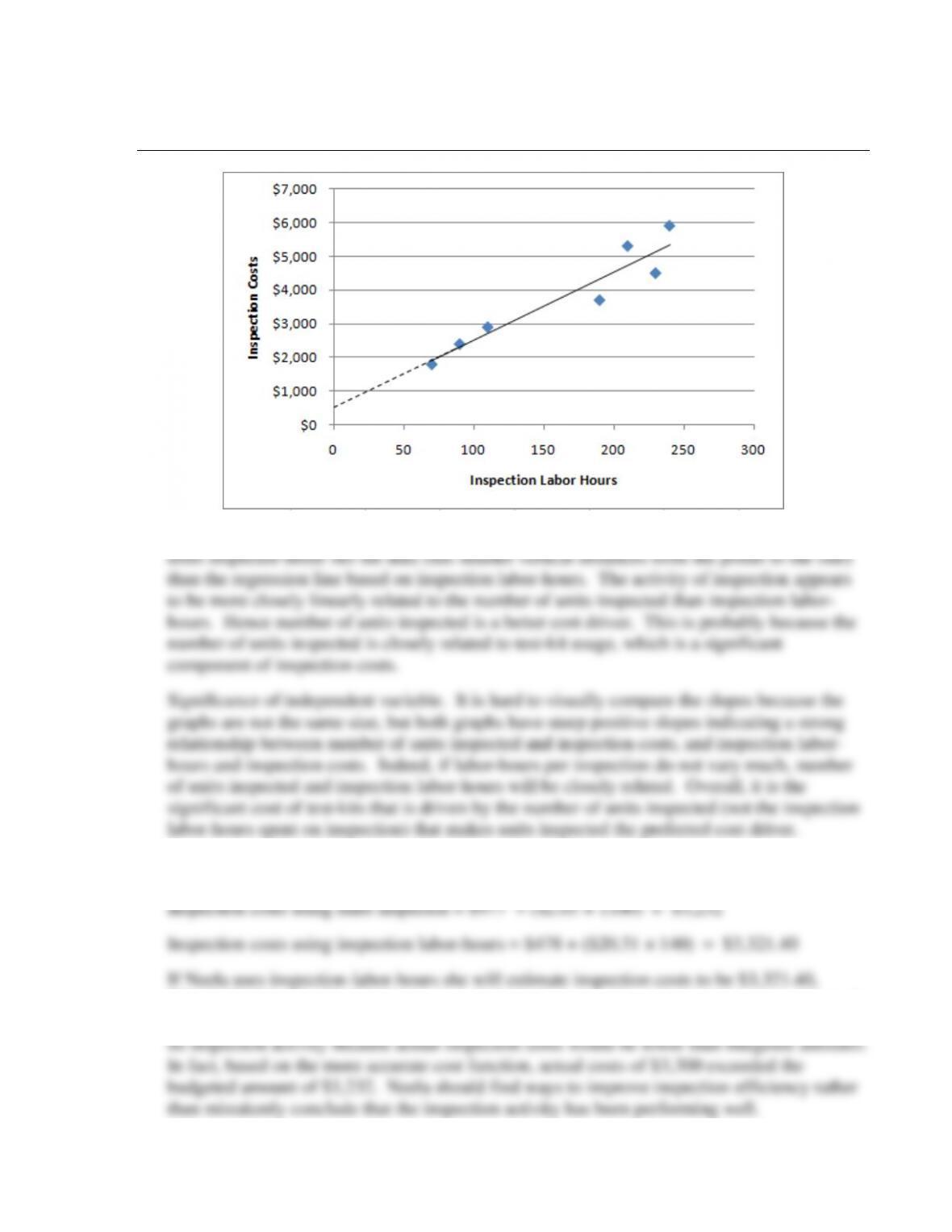
versus inspection costs and (b) the plots and regression line for inspection labor-hours and
10-27
SOLUTION EXHIBIT 10-34B
Plot and Regression Line for Inspection Labor-Hours and Inspection Costs for Fitzgerald
Manufacturing
Goodness of Fit. As you can see from the two graphs, the regression line based on number of
3. At 140 inspection labor hours and 1100 units inspected,
$89.40 ($3,321.40 ─$3,232) higher than if she had used number of units inspected. If actual
costs equaled, say, $3,300, Neela would conclude that Fitzgerald has performed efficiently in
10-28
10-35 (15-20 min.) Interpreting regression results, matching time periods.
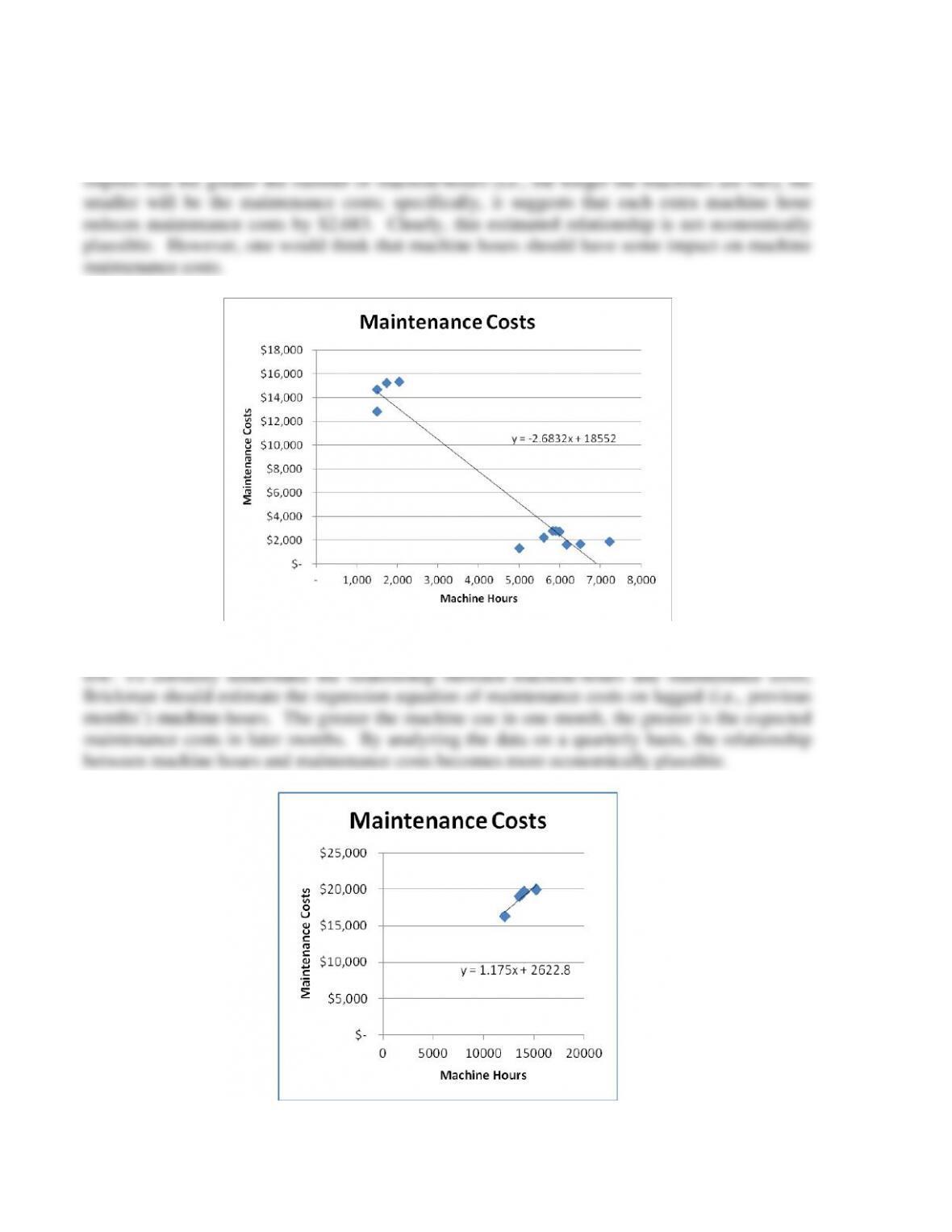
1. Sascha Green is commenting about some surprising and economically–implausible
regression results. In the regression, the coefficient on machine-hours has a negative sign. This
2. The problem statement tells us that Brickman has four peak sales periods, each lasting
two months and it schedules maintenance in the intervening months, when production volume is
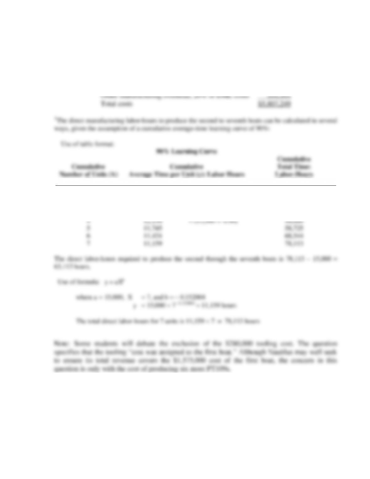
10-36 (30–40 min.) Cost estimation, cumulative average-time learning curve.
1. Cost to produce the 2nd through the 7th troop deployment boats:
Direct materials, 6
$200,000
$1,200,000
Direct manufacturing labor (DML), 63,1131
$40
2,524,520
Variable manufacturing overhead, 63,113
$25
1,577,825
Other manufacturing overhead, 20% of DML costs
504,904
Total costs
$5,807,249
10-30
2. Cost to produce the 2nd through the 7th boats assuming linear function for direct labor–
hours and units produced:
Direct materials, 6
$200,000
$1,200,000
Direct manufacturing labor (DML), 6
15,000 hrs.
$40
3,600,000
Variable manufacturing overhead, 6
15,000 hrs.
$25
2,250,000
Other manufacturing overhead, 20% of DML costs
720,000
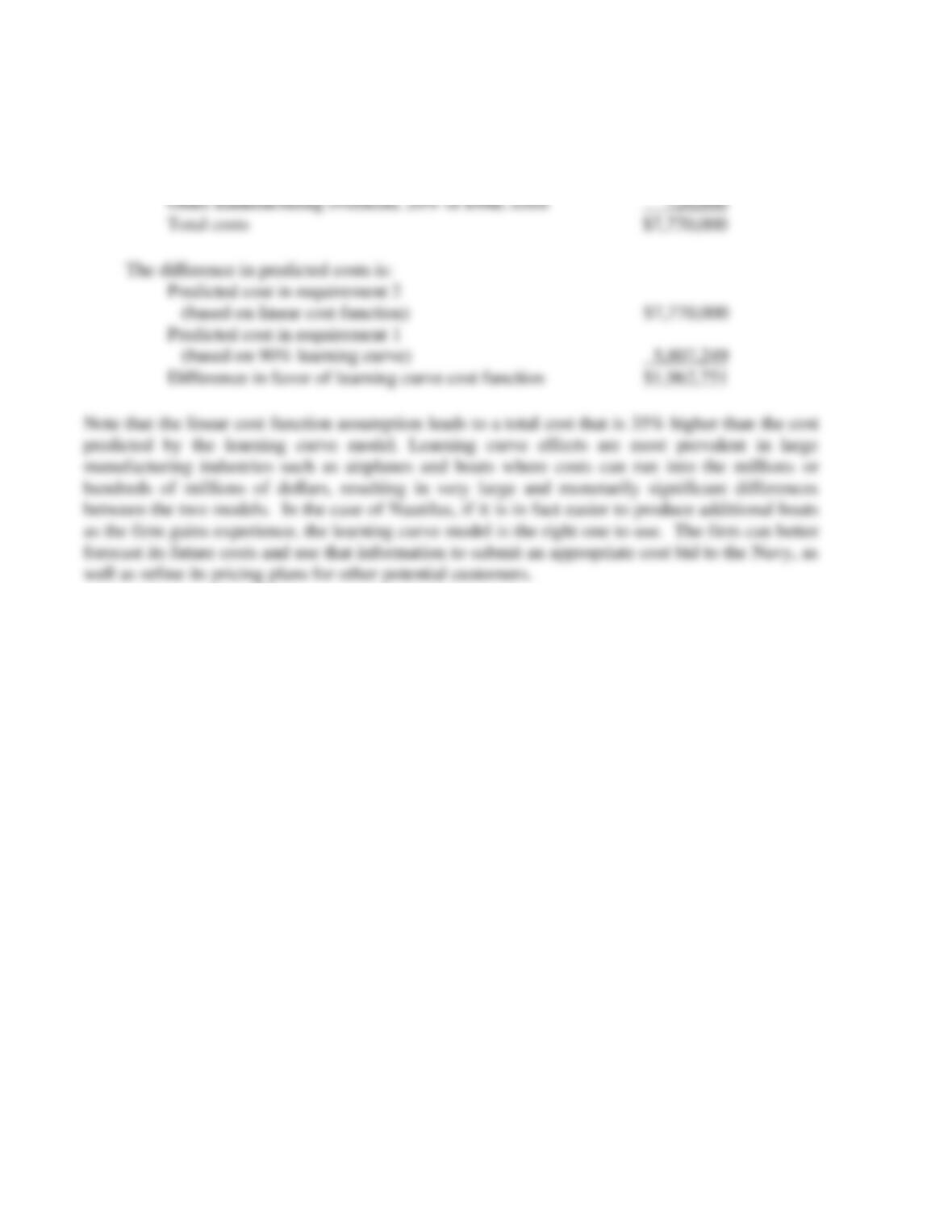
Total costs
$7,770,000
The difference in predicted costs is:
Predicted cost in requirement 2
(based on linear cost function)
$7,770,000
Predicted cost in requirement 1
(based on 90% learning curve)
5,807,249
Difference in favor of learning curve cost function
$1,962,751
Note that the linear cost function assumption leads to a total cost that is 35% higher than the cost
predicted by the learning curve model. Learning curve effects are most prevalent in large
manufacturing industries such as airplanes and boats where costs can run into the millions or
hundreds of millions of dollars, resulting in very large and monetarily significant differences
between the two models. In the case of Nautilus, if it is in fact easier to produce additional boats
as the firm gains experience, the learning curve model is the right one to use. The firm can better
forecast its future costs and use that information to submit an appropriate cost bid to the Navy, as
well as refine its pricing plans for other potential customers.