10-11
1. Slope coefficient (b) = Difference in cost
Difference in labor-hours =
$533,000 $400,000
6,500 3,000
−
−
= $38.00
7,500. The constant component provides the best available starting point for a straight line that
approximates how a cost behaves within the 2,000 to 7,500 relevant range.
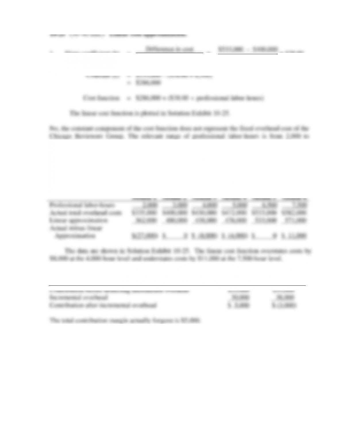
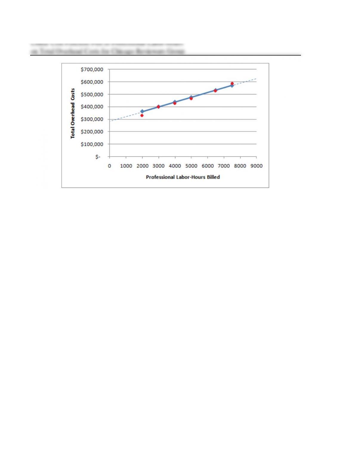
2. A comparison at various levels of professional labor-hours follows. The linear cost function
is based on the formula of $286,000 per month plus $38.00 per professional labor-hour.
Total overhead cost behavior:
Month 1
Month 2
Month 3
Month 4
Month 5
Month 6
Professional labor-hours
Actual total overhead costs
Linear approximation
Actual minus linear
Approximation
2,000
$335,000
362,000
$(27,000)
3,000
$400,000
400,000
$ 0
4,000
$430,000
438,000
$ (8,000)
5,000
$472,000
476,000
$ (4,000)
6,500
$533,000
533,000
$ 0
7,500
$582,000
571,000
$ 11,000
The data are shown in Solution Exhibit 10-25. The linear cost function overstates costs by
$8,000 at the 4,000-hour level and understates costs by $11,000 at the 7,500-hour level.
3. Based on Based on Linear
Actual Cost Function
10-12
SOLUTION EXHIBIT 10-25
10-13
10-26 (20 min.) Cost-volume-profit and regression analysis.
1a. Average cost of manufacturing =
Total manufacturing costs
Number of bicycle frames
$1,056,000
32,000
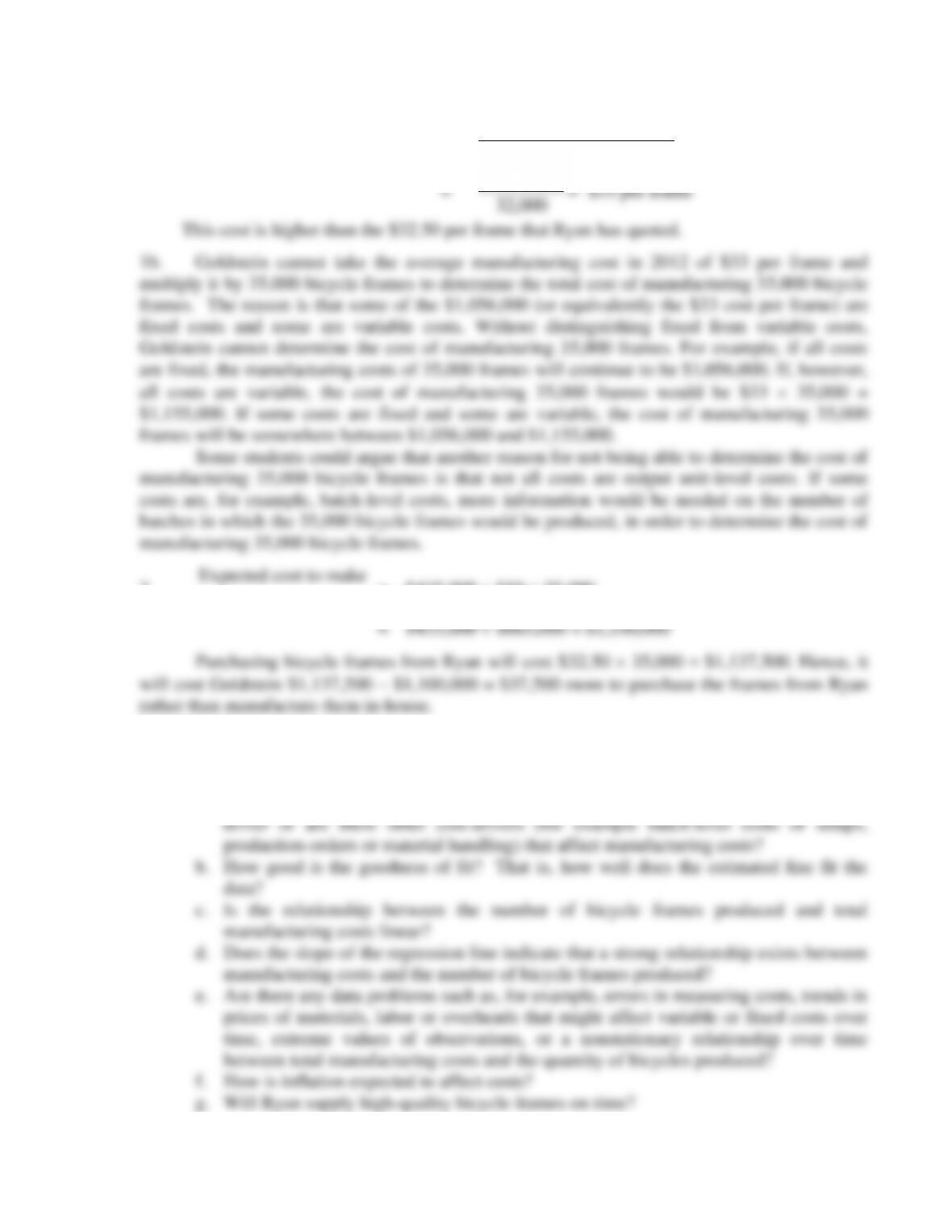
This cost is higher than the $32.50 per frame that Ryan has quoted.
1b. Goldstein cannot take the average manufacturing cost in 2012 of $33 per frame and
multiply it by 35,000 bicycle frames to determine the total cost of manufacturing 35,000 bicycle
frames. The reason is that some of the $1,056,000 (or equivalently the $33 cost per frame) are
fixed costs and some are variable costs. Without distinguishing fixed from variable costs,
Goldstein cannot determine the cost of manufacturing 35,000 frames. For example, if all costs
are fixed, the manufacturing costs of 35,000 frames will continue to be $1,056,000. If, however,
all costs are variable, the cost of manufacturing 35,000 frames would be $33 35,000 =
$1,155,000. If some costs are fixed and some are variable, the cost of manufacturing 35,000
frames will be somewhere between $1,056,000 and $1,155,000.
Some students could argue that another reason for not being able to determine the cost of
manufacturing 35,000 bicycle frames is that not all costs are output unit-level costs. If some
costs are, for example, batch-level costs, more information would be needed on the number of
batches in which the 35,000 bicycle frames would be produced, in order to determine the cost of
manufacturing 35,000 bicycle frames.
2.
Expected cost to make
35,000 bicycle frames
= $435,000 + $19 35,000
3. Goldstein would need to consider several factors before being confident that the equation
in requirement 2 accurately predicts the cost of manufacturing bicycle frames.
a. Is the relationship between total manufacturing costs and quantity of bicycle frames
economically plausible? For example, is the quantity of bicycles made the only cost
10-14
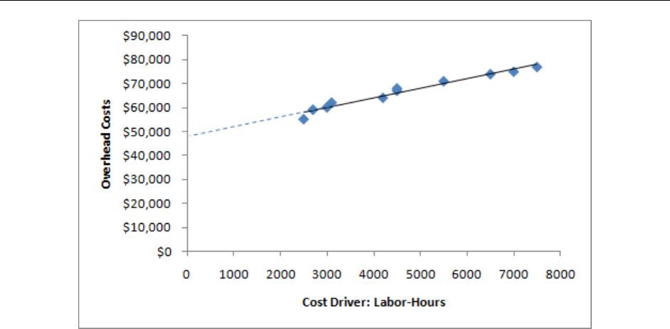
1. Solution Exhibit 10-27 plots the relationship between labor-hours and overhead costs and
shows the regression line. y = $48,271 + $3.93 X
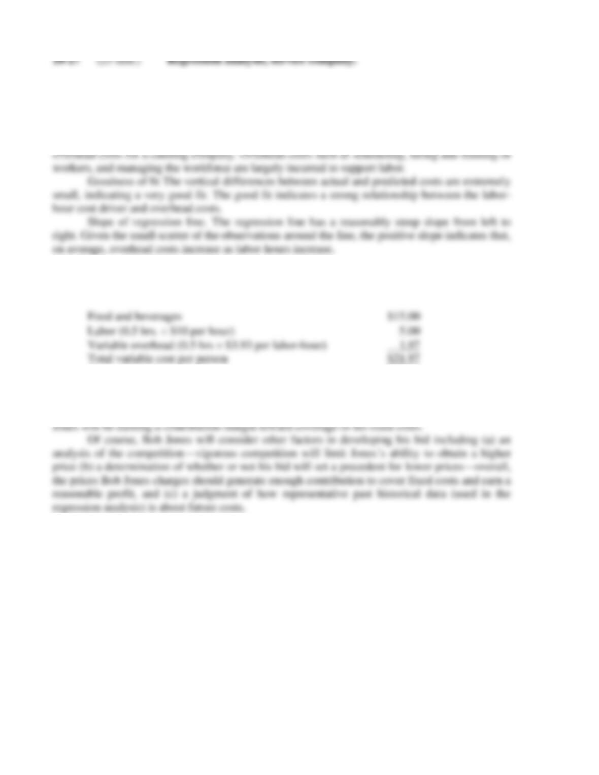
Economic plausibility. Labor-hours appears to be an economically plausible driver of
2. The regression analysis indicates that, within the relevant range of 2,500 to 7,500 labor–
hours, the variable cost per person for a cocktail party equals:
3. To earn a positive contribution margin, the minimum bid for a 200-person cocktail party
would be any amount greater than $4,394. This amount is calculated by multiplying the variable
cost per person of $21.97 by the 200 people. At a price above the variable costs of $4,394, Bob
10-15
SOLUTION EXHIBIT 10-27
Regression Line of Labor-Hours on Overhead Costs for Bob Jones’s Catering Company
10-16
10-28 High-low, regression
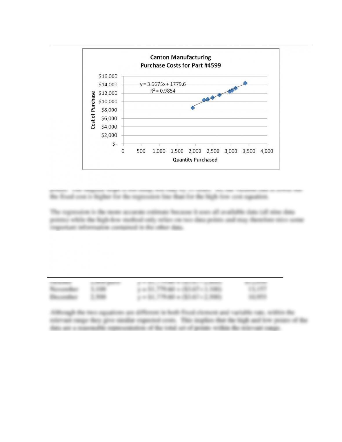
1. Melissa will pick the highest point of activity, 3,390 parts (March) at $14,400 of cost, and the
lowest point of activity, 1,930 parts (August) at $8,560.
Cost driver:
Quantity Purchased
Cost
Highest observation of cost driver
3,390
$14,400
Lowest observation of cost driver
1,930
8,560
Difference
1,460
$ 5,840
Purchase costs = a + b
Quantity purchased
Slope Coefficient =
$5,840
1,460
= $4 per part
Constant (a) = $14,400 ─ ($4
3,390) = $840
The equation Melissa gets is:
Purchase costs = $840 + ($4
Quantity purchased)
2. Using the equation above, the expected purchase costs for each month will be:
Month
Purchase
Quantity
Expected
Formula
Expected cost
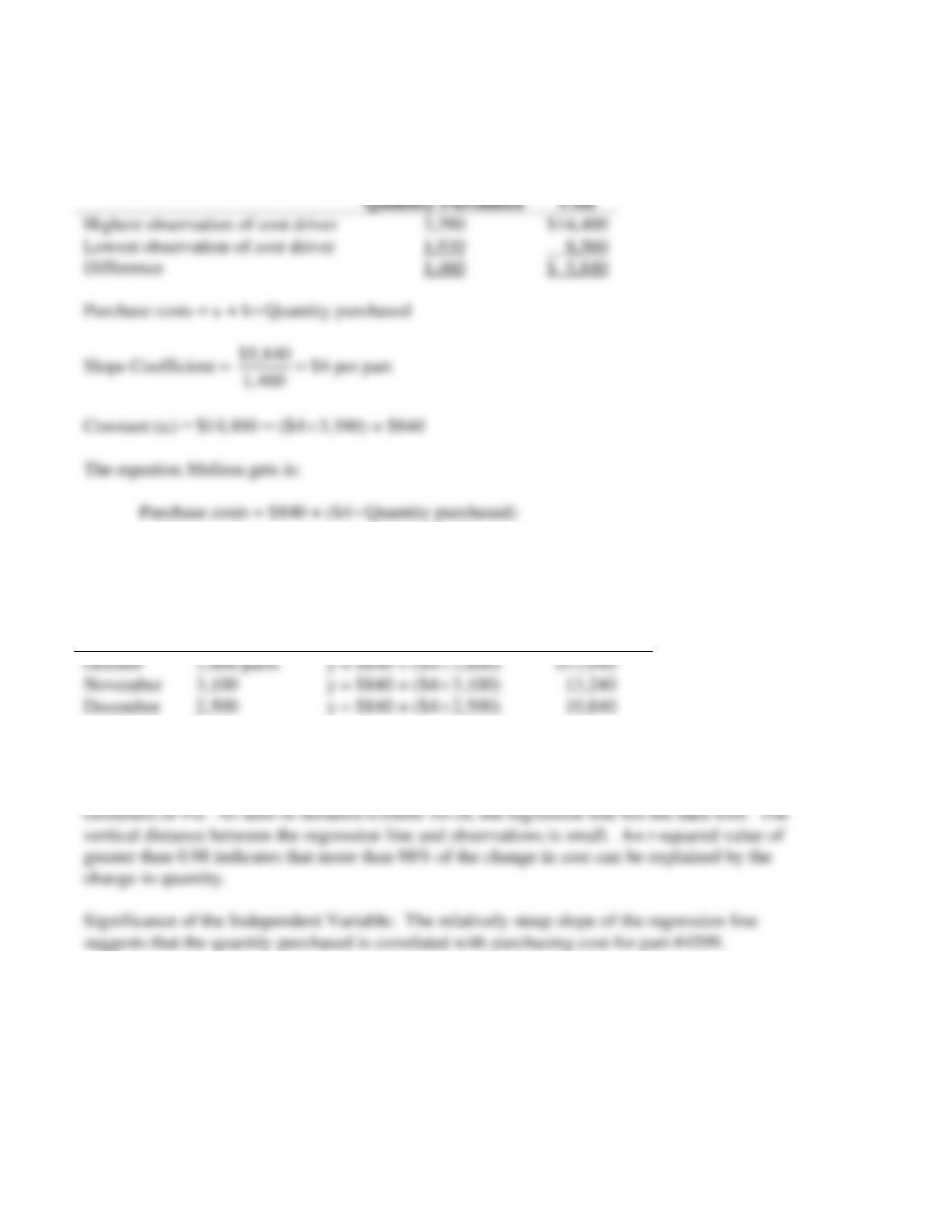
3. Economic Plausibility: Clearly, the cost of purchasing a part is associated with the quantity
purchased.
10-17
SOLUTION EXHIBIT 10-28
According to the regression, Melissa’s original estimate of fixed cost is too low given all the data
4. Using the regression equation, the purchase costs for each month will be:
Month
Purchase
Quantity
Expected
Formula
Expected cost
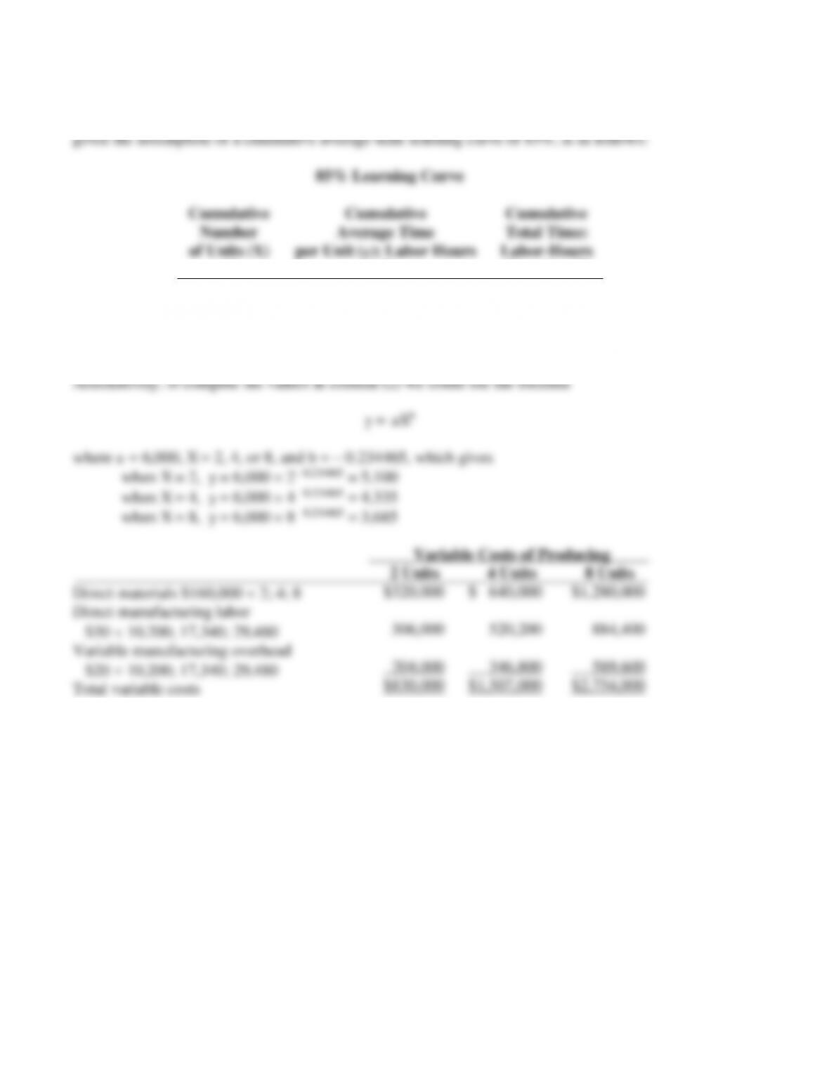
10-29 (20 min.) Learning curve, cumulative average-time learning model.
The direct manufacturing labor-hours (DMLH) required to produce the first 2, 4, and 8 units
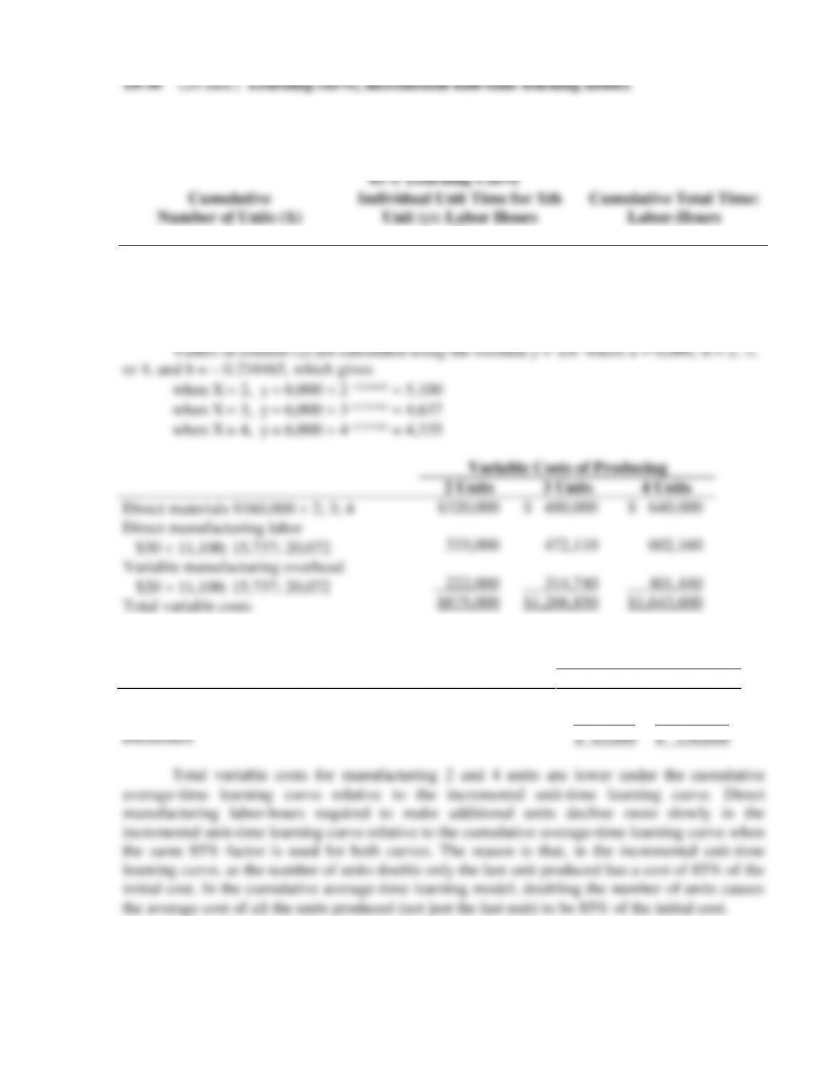
1. The direct manufacturing labor-hours (DMLH) required to produce the first 2, 3, and 4
units, given the assumption of an incremental unit–time learning curve of 85%, is as follows:
85% Learning Curve
Cumulative
Number of Units (X)
Individual Unit Time for Xth
Unit (y): Labor Hours
Cumulative Total Time:
Labor-Hours
(1)
(2)
(3)
1
6,000
6,000
2
5,100
= (6,000
0.85)
11,100
3
4,637
15,737
4
4,335
= (5,100
0.85)
20,072
$ 45,000
10-20
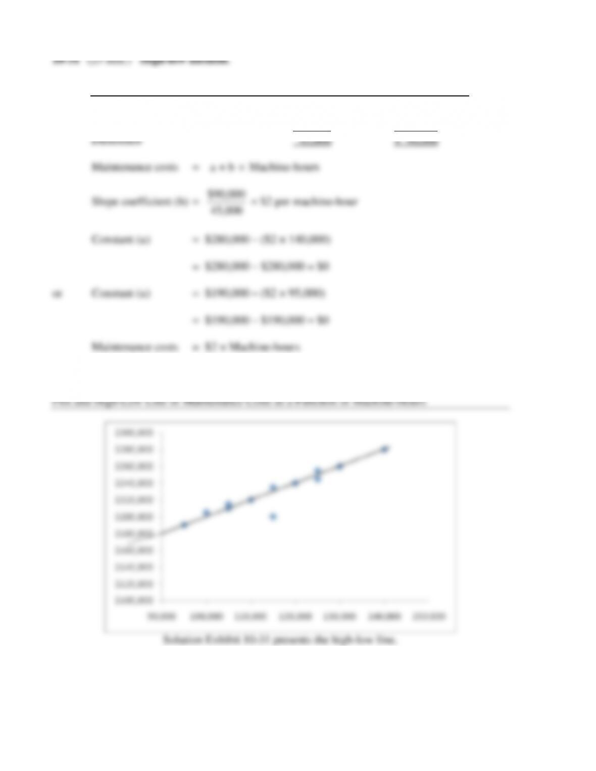
1. Machine-Hours Maintenance Costs
Highest observation of cost driver 140,000 $280,000
Lowest observation of cost driver 95,000 190,000
2.
SOLUTION EXHIBIT 10-31