111
Solution to Problems in Chapter 8, Section 8.6
8.1. The total volume of a 70-kg human body is approximately 70 liters. Therefore, the volume
fraction of the vascular compartment is 6/70 or 8.6%.
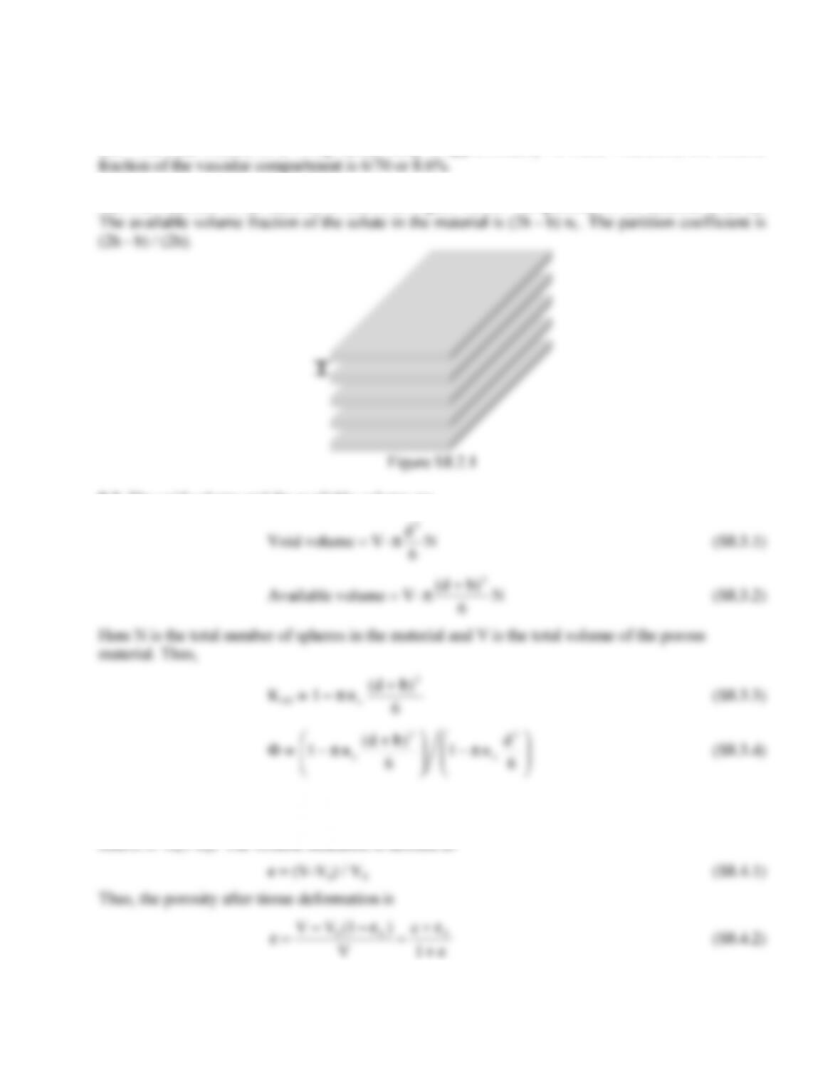
8.2. The structure of the material is shown in Figure S8.2.1. The porosity of the material is 2h nL.
The available volume fraction of the solute in the material is (2h – b) nL. The partition coefficient is
Void volume = V-
N
6
d3
π
(S8.3.1)
8.4. Assume the initial volume of the tissue is V0. Then the total volume of cells and extracellular
matrix is V0(1-ε0). The volume dilatation is defined as
e = (V-V0) / V0 (S8.4.1)
8.5. (a) The porosity of the tissue is
112
ε =
4
d
6
d
n1
2
f
3
c
vπ−π−
(S8.5.1)
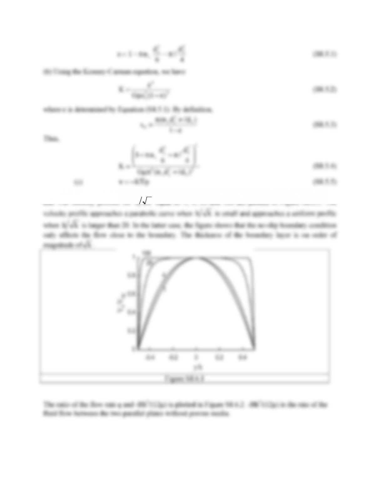
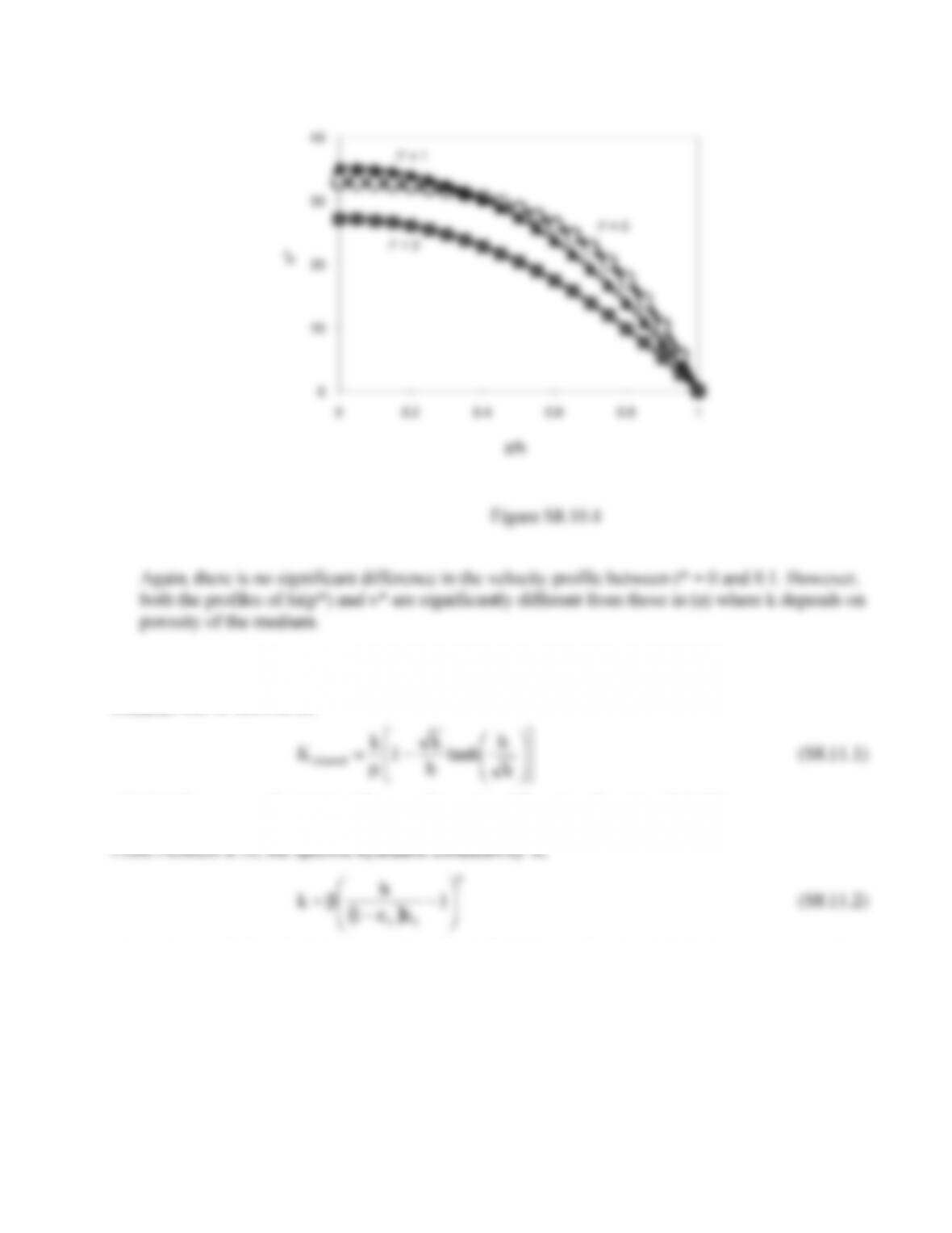
8.6. The velocity profiles for
kh
equal to 1, 4, 20 and 100 are plotted in Figure S8.6.1. The
113
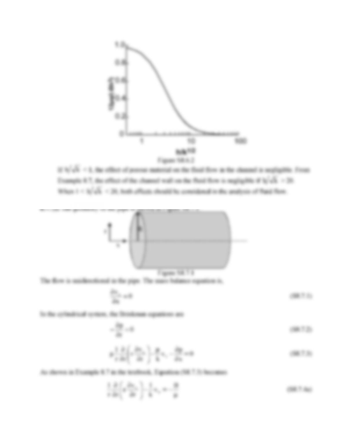
Figure S8.6.2
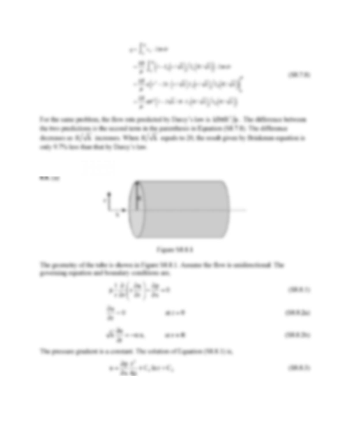
8.7. (a) The geometry of the pipe is shown in Figure S8.7.1.
114
Here -B is the pressure gradient in x direction, (p2-p1) / L. The boundary conditions of Equation
(S8.7.4) are
0
r
vx=
∂
∂
at r = 0 (S8.7.4b)
0v x=
at r = R (S8.7.4c)
To solve Equation (S8.7.4), we substitute vx with v’+kB/µ. Therefore, Equation (S8.7.4) and the
boundary conditions become,
0‘v
k
1
r
‘v
r
rr
1=−
⎟
⎟
⎠
⎞
⎜
⎜
⎝
⎛
∂
∂
∂
∂
(S8.7.5)
0
r
‘v =
∂
∂
at r = 0 (S8.7.5a)
µ
−=kB
‘v
at r = R (S8.7.5b)
The solution of Equation (S8.7.5) is
v‘ =−kB
µ
I0r / k
( )
I0R / k
( )
(S8.7.6)
Here
I0r / k
( )
is the zeroth order modified Bessel function of
k/r
. Thus, the solution of vx is
vx=kB
µ
1−I0r / k
( )
I0R / k
( )
( )
(S8.7.7)
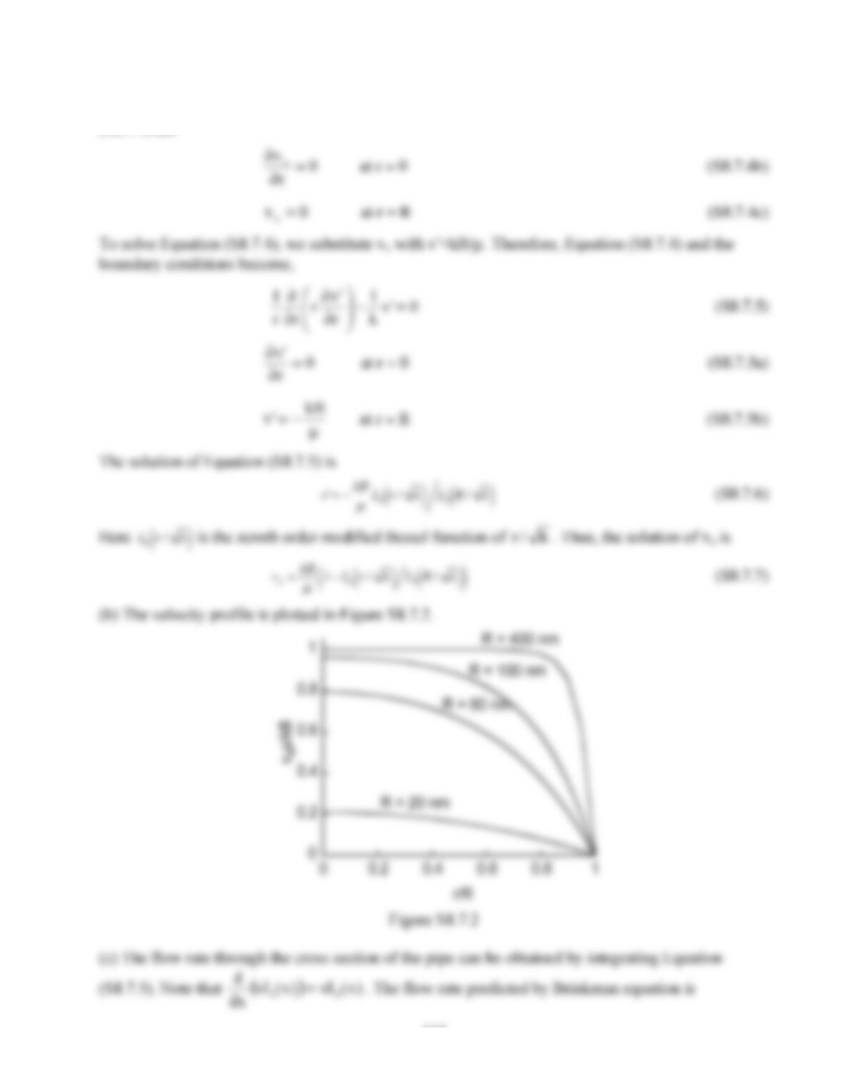
(b) The velocity profile is plotted in Figure S8.7.2.
Figure S8.7.2
(c) The flow rate through the cross section of the pipe can be obtained by integrating Equation
(S8.7.5). Note that
( ) )x(xI)x(xI
dx
d
01 =
. The flow rate predicted by Brinkman equation is
115
q=vx⋅2
π
rdr
0
R
∫
=kB
µ
1−I0r / k
( )
I0R / k
( )
( )
⋅2
π
rdr
0
R
∫
=kB
µπ
r2−2k ⋅r / k
( )
I1r / k
( )
I0R / k
( )
( )
0
R
=kB
µπ
R21−2 k / R ⋅I1R / k
( )
I0R / k
( )
( )
(S8.7.8)
For the same problem, the flow rate predicted by Darcy’s law is
µπ2
RkB
. The difference between
the two predictions is the second term in the parenthesis in Equation (S8.7.8). The difference
decreases as
kR
increases. When
kR
equals to 20, the result given by Brinkman equation is
only 9.7% less than that by Darcy’s law.
8.8. (a)
C1 and C2 are constants, which can be determined by applying the boundary conditions. The final
solution is
116
( ) x
p
2
Rk
Rr
x
p
4
1
u22
∂
∂
µα
−−
∂
∂
µ
=
(S8.8.4)
(b) The flow rate q is
⎟
⎟
⎠
⎞
⎜
⎜
⎝
⎛
µ
π
α
+
µ
π
∂
∂
−=
π⋅=∫
2
Rk
8
R
x
p
rdr2uq
34
R
0
(S8.8.5)
According to Equation (S8.8.5), the slip effect reduces the pressure gradient by a factor of
R
k4
1
α
+
, if the flow rate is fixed.
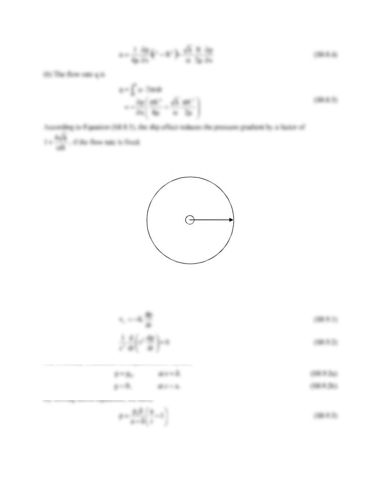
8.9.
r
Figure S8.9.1
The fluid flow is spherically symmetric. Therefore, the velocity is unidirectional along the radial
direction. In this case, the spherical coordinate system is used, in which Equations (8.3.2) and (8.3.3)
become,
dr
dp
Kvr−=
(S8.9.1)
0
dr
dp
r
dr
d
r
12
2=
⎟
⎠
⎞
⎜
⎝
⎛
(S8.9.2)
The boundary conditions for Equation (S8.9.2) are,
p = p0, at r = δ. (S8.9.2a)
117
2
0
rr
K
a
ap
vδ−
δ
=
(S8.9.4)
(b). The infusion rate can be obtained by integrating the velocity at the surface of the fluid cavity.
δ−
δπ
=πδ=φθθδ=∫∫
π π
a
Kap4
v4ddsinvq 0
r
22
2
0 0
r
(S8.9.5)
i.e., q = 4πr2vr at any location.
8.10. (a) The half distance h is a function of time,
( )
[ ]
t
00
t
0h0 e11hdtVhh α−
−ε−=−=∫
(S8.10.1)
The tissue dilatation is
0
0
h
hh
e−
=
(S8.10.2)
Substitute the above equation into Equation (S8.4.2), we have,
( ) h
h
11
e1
e0
0
0ε−−=
+
ε+
=ε
(S8.10.3)
The specific hydraulic conductivity is,
( )
n
0
t
0
n
00
n
1
1
)e1(1
1
h1
h
1
k⎟
⎟
⎠
⎞
⎜
⎜
⎝
⎛−
ε−
−ε−
β=
⎟
⎟
⎠
⎞
⎜
⎜
⎝
⎛−
ε−
β=
⎟
⎠
⎞
⎜
⎝
⎛
ε−
ε
β=
α−
(S8.10.4)
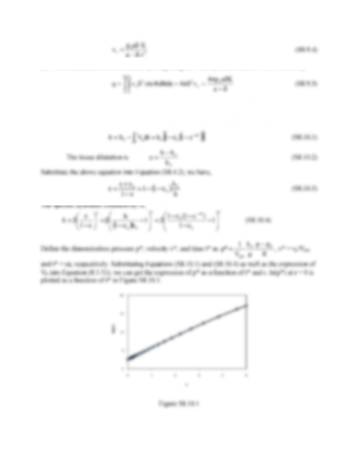
Define the dimensionless pressure p*, velocity v*, and time t* as
R
ppk
V
1
*p 00
0h
−
µ
=
, v* = vr/Vh0,
and t* = αt, respectively. Substituting Equations (S8.10.1) and (S8.10.4) as well as the expression of
Vh into Equation (8.3.51), we can get the expression of p* as a function of t* and r. ln(p*) at r = 0 is
plotted as a function of t* in Figure S8.10.1.
Figure S8.10.1
0
5
10
15
20
0 1 2 3 4 5
ln(p*)
t*
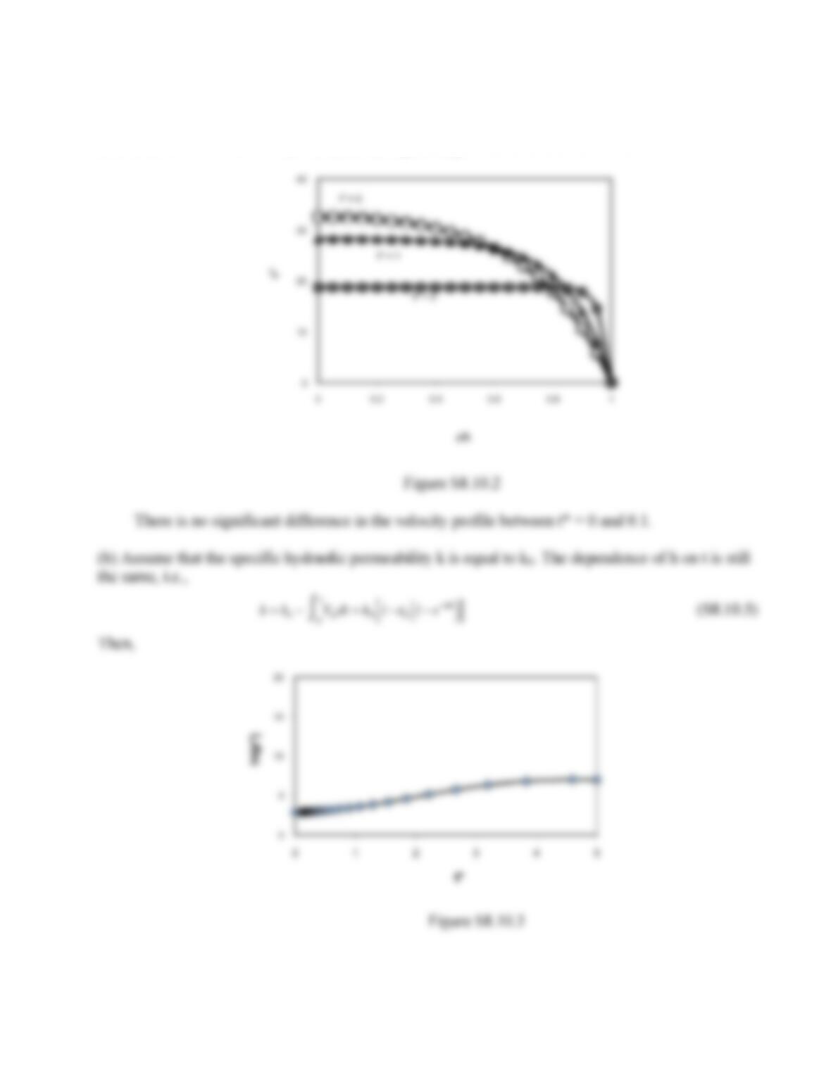
Similarly, Substituting Equations (S8.10.1) and (S8.10.4) as well as the expression of Vh into
Equation (8.3.52), we can get the expression of v* as a function of t*, r, and z. v* at r = R is plotted
as a function of z/h for t* = 0, 0.1, 1, and 3, respectively.
Figure S8.10.2
0
10
20
30
40
0 0.2 0.4 0.6 0.8 1
v*
z/h
t* = 3
t* = 1
t* = 0
119
Figure S8.10.4
8.11. Using Equations (8.3.51) and (8.3.52), the effective hydraulic conductivity in the channel
(Kchannel) can be derived as,
⎥
⎦
⎤
⎢
⎣
⎡⎟
⎠
⎞
⎜
⎝
⎛
−
µ
=k
h
tanh
h
k
1
k
Kchannel
(S8.11.1)
which is the same as that derived for one-dimensional flow (see Equation (8.3.41)).
From Problem 8.10, the specific hydraulic conductivity is,
where (1 – ε0) ≤ h/ h0 ≤.1. Substituting Equation (S8.11.2) into Equation (S8.11.1) and assuming the
values of constants to be the same as those in Problem 8.10, we can plot Kchannel/(k0/µ) as a function
of h/h0.
0
10
20
30
40
0 0.2 0.4 0.6 0.8 1
v*
z/h
t* = 3
t* = 1
t* = 0

120
8.12.
Drug transport in the tissues can be considered by a one-dimensional diffusion, since the diameter of
the polymer membrane is much larger than its thickness. Therefore, the mass balance equation of the
drug is,
Before the membrane is implanted, there is no drug in the tissues. Thus, the initial condition is,
C = 0, when t = 0 (S8.12.2)
The concentration of the drug at the surface of the membrane is assumed to be C0. We also assume
that the tissue is infinitely large in the x-direction since its dimension is much larger than the
thickness of the membrane. In this case, the boundary conditions are,
C = C0, at x = 0 (S8.12.3)
121
Based on Equation (6.8.18), the solution of C can be obtained as,
⎟
⎟
⎠
⎞
⎜
⎜
⎝
⎛
=
tD4
x
erfcCC
eff
0
(S8.12.5)
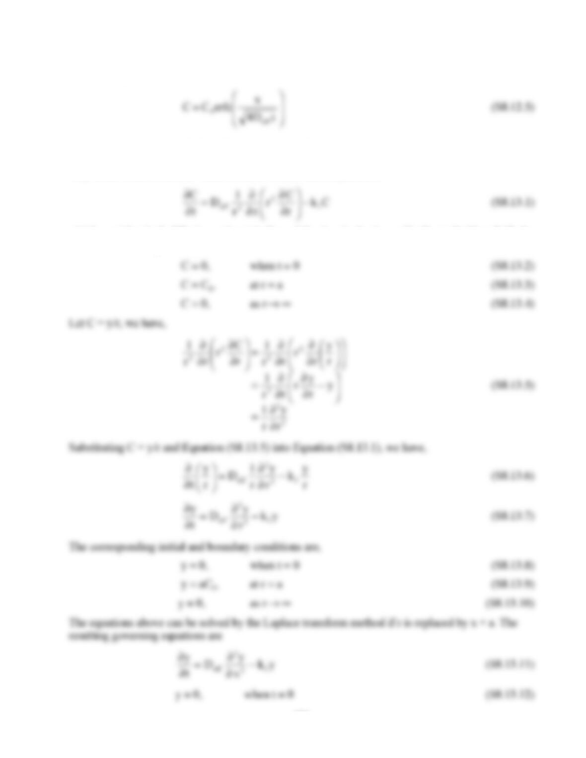
8.13. For the spherical implant, it is more convenient to use spherical coordinates. The diffusion is
only in the radial direction. Thus, the mass conservation equation is
Ck
r
C
r
r
r
1
D
t
C
f
2
2
eff −
⎟
⎟
⎠
⎞
⎜
⎜
⎝
⎛
∂
∂
∂
∂
=
∂
∂
(S8.13.1)
which considers both diffusion and metabolism of the drug in the tissue. Similar to Problem 8.12, the
initial and boundary conditions are,
C = 0, when t = 0 (S8.13.2)
122
y = aC0, at x = 0 (S8.13.13)
( )
∫ττ−
⎟
⎟
⎠
⎜
⎜
⎝
τ
+
0f
eff
f0
dkexp
D4
erfckaC
123
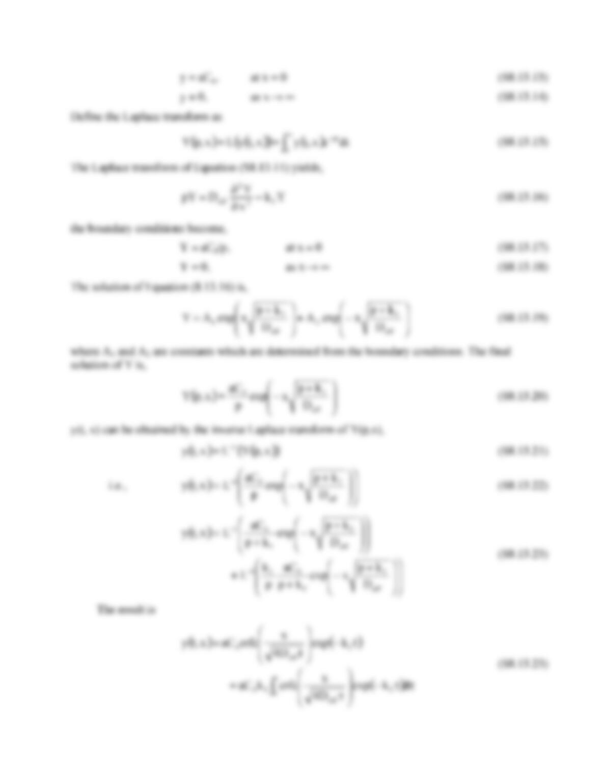
Therefore, the concentration C is,
( ) ( )
( )
∫ττ−
⎟
⎟
⎠
⎞
⎜
⎜
⎝
⎛
τ
−
+
−
⎟
⎟
⎠
⎞
⎜
⎜
⎝
⎛−
=
t
0f
eff
f0
f
eff
0
dkexp
D4
ar
erfc
r
kaC
tkexp
tD4
ar
erfc
r
aC
r,tC
(S8.13.24)
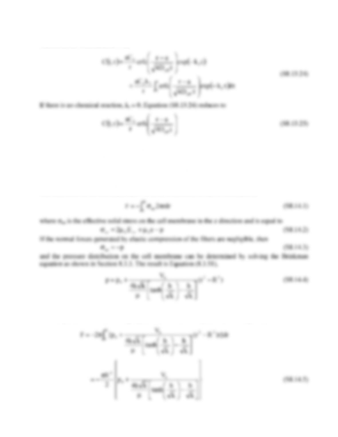
If there is no chemical reaction, kf = 0, Equation (S8.13.24) reduces to
( ) ⎟
⎟
⎠
⎞
⎜
⎜
⎝
⎛−
=tD4
ar
erfc
r
aC
r,tC
eff
0
(S8.13.25)
8.14. To simplify, assume that the extracellular matrix is highly compressible compared with the
intracellular volume. Therefore, the normal forces generated by elastic compression of the fibers are
negligible compared to the pressure generated within the porous layer. Without this assumption, the
problem can still be solved, but it is too difficult for most undergraduate students.
The total force on the cell membrane F is in the z direction. It can be calculated as
∫πσ−=
R
0zz rdr2F
(S8.14.1)
k
k
tanh
⎥
⎦
⎢
⎣
⎟
⎠
⎜
⎝
µ
It is independent of z. Substituting Equation (S8.14.4) into Equation (S8.14.1) yields,
∫−
⎤
⎡−
⎞
⎛
+π−=R
0
22
h
0dr}r)Rr(
h
h
kk4
V
p{2F
⎪
⎭
⎪
⎩
⎥
⎦
⎢
⎣
⎟
⎠
⎜
⎝
µ
k
k
tanh
124
125
Solution to Problems in Chapter 9, Section 9.6
9.1. From Equation (9.3.36),
( )
( )
e
eLi
fvs Pexp1
PexpCC
)1(JJ −
−
σ−=
(9.3.36)
Substitute Ci with –ΔC+CL, we have
( )
( )
( )⎟
⎟
⎠
⎞
⎜
⎜
⎝
⎛
−
Δ
−−=
−
−+Δ−
−=
e
Lfv
e
eLL
fvs
P
C
CJ
P
PCCC
JJ
exp1
)1(
exp1
exp
)1(
σ
σ
(9.3.37)
Expand Equation (9.3.37) and substitute Jv(1-σf) with Pe PS in the second term,
( )
( ) 1exp
)1(
exp1
)1()1(
−
Δ
+−=
−
Δ
−−−=
e
e
Lfv
e
fvLfvs
P
CPSP
CJ
P
C
JCJJ
σ
σσ
(9.3.38)
Substitute CL with (CL+Ci+ΔC)/2 in the first term in Equation (9.3.38), we have
( )
( )
( )( )
( ) ⎭
⎬
⎫
⎩
⎨
⎧
−
+Δ−
+
+
−=
⎟
⎟
⎠
⎞
⎜
⎜
⎝
⎛
−
Δ
−
Δ
−+
+
−=
−
Δ
−−
Δ
−+
+
−=
1exp
1exp)1(
2
1
2
)1(
exp12
)1(
2
)1(
exp1
)1(
2
)1(
2
)1(
e
efv
iL
fv
e
fv
iL
fv
e
fvfv
iL
fvs
P
PCJ
CC
J
P
CC
J
CC
J
P
C
J
C
J
CC
JJ
σ
σ
σσ
σσσ
(9.3.39)
9.2. The thickness of a membrane is very small. As a result, the transport of the solute can reach
steady state rapidly. Therefore, the flux of the solute in the membrane can be calculated based on the
steady state mass balance equation,
2
2
0
x
C
DA∂
∂
=
(S9.2.1)
where C is the concentration of solute in the membrane. At the surface of the porous membrane, the
continuity of the concentration is,
C = C1 KA, at x = 0 (S9.2.2a)
C = C2 KA, at x = L (S9.2.2b)
By solving Equation (S9.2.1) with its boundary conditions, we obtain,
( ) L
x
CKCK
L
x
CCKCKC AAAA Δ−=−+= 1121
(S9.2.3)
126
The flux of solute in the membrane is
L
C
KD
x
C
DJ AAAs
Δ
=
∂
∂
−=
(S9.2.4)
Therefore, the permeability of the membrane is
LKDP AA /=
(S9.2.5)
9.3. (a) For an electrolyte, the mass balance equation is (see Sec. 7.4),
⎟
⎟
⎠
⎞
⎜
⎜
⎝
⎛
∂
Ψ∂
⎟
⎠
⎞
⎜
⎝
⎛
+
∂
∂
∂
∂
=
xRT
F
Cz
x
C
D
xBB
0
(S9.3.1)
Here
Lx
12 Ψ−Ψ
=
∂
Ψ∂
. The boundary conditions for Equation S9.3.1 are,
C = C1 KB, at x = 0 (S9.3.2a)
C = C2 KB, at x = L (S9.3.2b)
The solution of Equation (S9.3.1) is
( ) ⎪
⎭
⎪
⎬
⎫
⎪
⎩
⎪
⎨
⎧⎥
⎦
⎤
⎢
⎣
⎡−
⎟
⎟
⎠
⎞
⎜
⎜
⎝
⎛
⎥
⎦
⎤
⎢
⎣
⎡−
⎟
⎟
⎠
⎞
⎜
⎜
⎝
⎛
−+= 1exp1exp
121 L
D
E
x
D
E
CCCKC
BB
B
(S9.3.3)
where
( )
RTL
Fz
EB21 Ψ−Ψ
=
.
(b) The flux of the solute B in the membrane is,
⎥
⎦
⎤
⎢
⎣
⎡−
⎟
⎟
⎠
⎞
⎜
⎜
⎝
⎛
⎥
⎦
⎤
⎢
⎣
⎡−
⎟
⎟
⎠
⎞
⎜
⎜
⎝
⎛
=1expexp 21
BB
Bs D
E
C
D
E
CEKJ
(S9.3.4)
9.4. In each pore, the diffusion flux of the solute is
hCDJ s/Δ=
(S9.4.1)
Assume the pores are identical, the total flux of the solute through the vessel wall equals to the
diffusion flux in one pore times the surface area ratio of the pore,
h
CDdn
d
nJJ A
As 44
2
2Δ
=⋅=
π
π
(S9.4.2)
Therefore, the permeability of the vessel wall is,
h
Ddn
CJP A
4
/
2
π
=Δ=
(S9.4.3)
9.5. (a) The porosity of the porous clefts is
127
lrf
2
1
πε
−=
(S9.5.1)
(b) Using the Kozeny-Carman theory (Equation 8.3.27), the hydraulic conductivity of a fiber matrix
material is
K=rf
2
ε
3
4G
µ
(1−
ε
)2=1−
π
rf
2l
( )
3
4G
µ
(
π
r2l)2
(S9.5.2)
Here G is Kozeny constant. For fiber matrix materials, G is determined by Equation 8.3.28.
(c) First, we consider the flux in one cleft. According to Darcy’s law,
PKV ∇−=
(S9.5.3)
The width of the cleft is much less than its length. In this case, the flow in the cleft is semi-
unidirectional, i.e. the flow is always parallel to the wall of the cleft. The press gradient should also
be calculated along the route of the cleft. Therefore,
hPKV /Δ=
(S9.5.4)
Taken together, the flux across the vessel wall is,
J=1−
π
rf
2l
( )
3
4G
µ
(
π
r2l)2
ΔP
hAp
(S9.5.5)
9.6. In a spherical system, Equation (8.3.4) becomes
0
12
2=
⎟
⎟
⎠
⎞
⎜
⎜
⎝
⎛
∂
∂
∂
∂
r
p
r
r
r
(S9.6.1)
The boundary conditions for Equation (S9.6.1) are,
0
pp =
, at
br =
(S9.6.1a)
0=p
, at
∞→r
(S9.6.1a)
Integrate Equation S9.6.1 and apply the boundary conditions, we have,
rbpp /
0⋅=
(S9.6.2)
The velocity can be calculated by Darcy’s law,
2
0/rbKppKV =∇−=
(S9.6.3)
In a spherical system, the mass balance equation (Equation 8.4.5) becomes,
( ) ⎟
⎟
⎠
⎞
⎜
⎜
⎝
⎛
∂
∂
∂
∂
=
∂
∂
r
C
r
r
r
DVCr
r
r
2
2
2
2
11
(S9.6.4)
The boundary conditions for above equation are,
ε
p
CC =
, at
br =
(S9.6.4a)
0=C
, at
∞→r
(S9.6.4a)
128
Here ε is the porosity of the subendothelial tissue. Solve Equation S9.6.4, we have,
⎥
⎦
⎤
⎢
⎣
⎡−
⎟
⎟
⎠
⎞
⎜
⎜
⎝
⎛−
⎥
⎦
⎤
⎢
⎣
⎡−
⎟
⎟
⎠
⎞
⎜
⎜
⎝
⎛−=1exp1exp 00
D
kp
rD
bkp
CC p
ε
(S9.6.5)
9.7. The fluorescence intensity is a linear function of the amount of the solute. Thus,
( )
b
IIA −=
α
(S9.7.1)
Here A is the total amount of the solute, α is a rate constant. The concentration of the solute in the
vessel can be estimated by,
( ) ( )
lrIIC bp
2
0/
πα
−=
(S9.7.2)
The concentration of the solute in the extravascular space is much smaller than that in the vessel.
Thus, the flow rate of the solute across the vessel wall is approximately,
rlCPQ papp
π
2⋅=
(S9.7.3)
The mass balance of the extravascular space is
( )( ) ( ) r
IIPQII
td
d
bapp
2
00 ⋅−==−
αα
(S9.7.4)
Rearrange the equation, we have
dt
dI
I
r
Papp
0
1
2Δ
=
(S9.7.5)
129
Solution to Problems in Chapter 10 Problem, Section 10.8
10.1. The generalized rate expression is:
R=kCA
aCB
b
(S10.1.1)
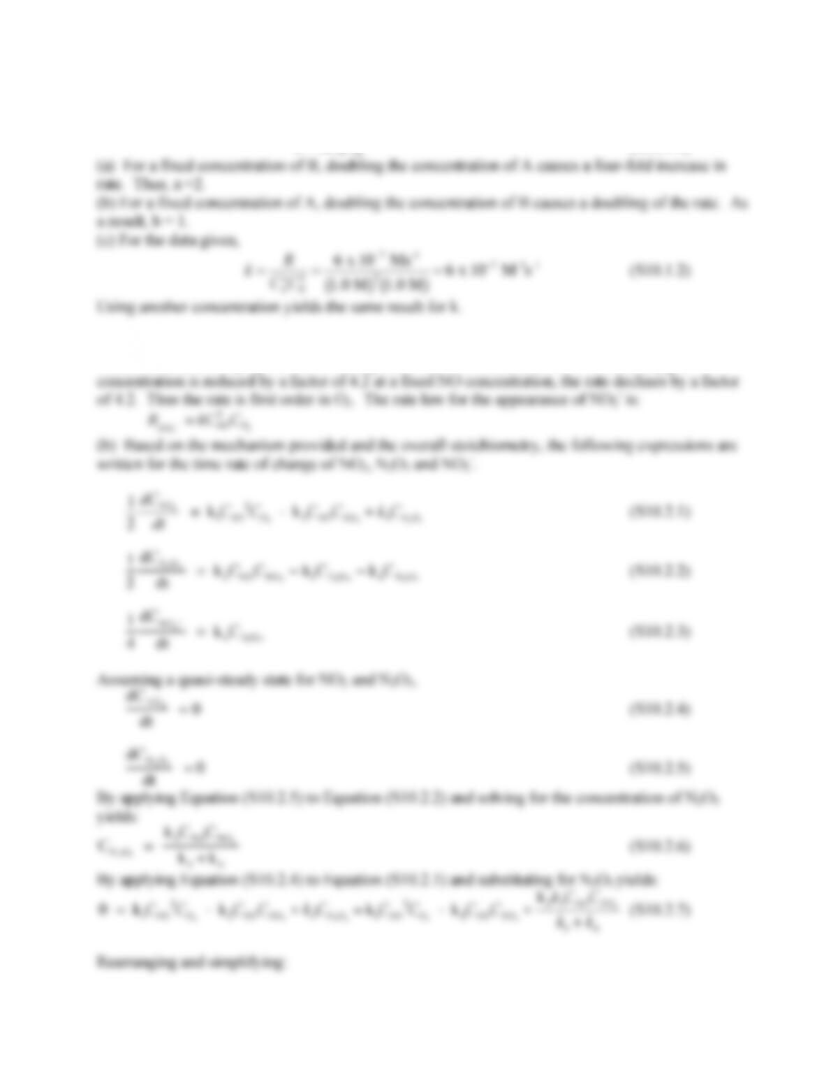
(a) For a fixed concentration of B, doubling the concentration of A causes a four-fold increase in
10.2. (a) For fixed O2, tripling the concentration of NO leads to a nine-fold increase in the rate.
Therefore, the rate is proportional to the square of the NO concentration. When the oxygen
concentration is reduced by a factor of 4.2 at a fixed NO concentration, the rate declines by a factor
130
0 =k1CNO
2CO2
+
–k3+k4
( )
k2CNOCNO2
+ k 2k3CNOCNO2
k3+k4
=k1CNO
2CO2
−
k4k2CNOCNO2
k3+k4
(S10.2.8)
Solving for NO2 yields the following relation:
CNO2=
k1k3+k4
( )
CNO CO2
k4k2
(S10.2.9)
Using equation (S10.2.9), the N2O3 concentration, equation (S10.2.6), can be expressed in terms of
the NO and O2 concentrations:
CN2O3
= k1
k4
CNO
2CNO 2
(S10.2.10)
Thus, the rate of appearance of NO2– is:
dCNO 2
−
dt
= 4k1CNO
2CNO 2
(S10.2.11)
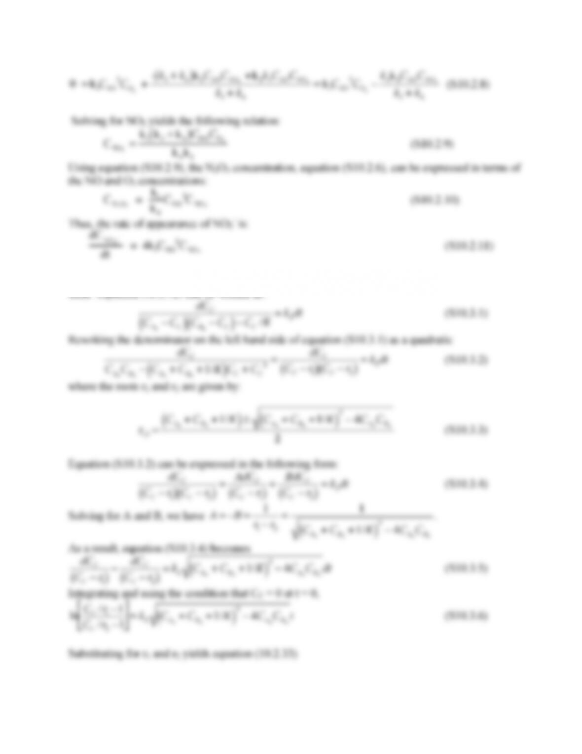
10.3. Equation (10.2.32) can be written as:
dCC
CA0
−CC
CB0
−CC
−CC/K=k2dt
(S10.3.1)
10.4. Rate expressions for the substrate, enzyme-substrate complex and product are: