Solution to Problems in Chapter 5, Section 5.11
5.1. (a) From Figure 5.11 one can write an expression for the variables that influence the pressure
drop:
Δp =f(ρ, µ, <v>, a, R, L)
There are seven dimensional groups and three dimensions (mass, length and time). Thus, there are,
at most, four dimensionless groups. These can be identified using the procedures outlined in Section
3.5.1. Alternatively, the groups can be identified from the known dimensionless groups. The
dimensionless pressure is Δp2a/(2ρ<v>2L) as is analogous to the group developed for flow in a
straight tube of diameter 2a and represents the product of two groups, Δp/(2ρ<v>2) and a/L. The
dimensionless pressure drop depends on two dimensionless groups. There are two possible
groupings. One is the Reynolds number and the ratio a/R. ALernatively, one could use the Dean
number and a/R.
5.2. Using Xe = 0.113RRe and Table 2.3, the following results are obtained for the lung.
Generation
Xe, cm, Quiet Breathing
Xe, cm, Vigorous Breathing
Trachea
236.4
948.3
1
118.5
474.0
and greater. For vigorous breathing, the length of the branch exceeds the entrance length for branch
generation 15 and greater.
69
5.3. (a) This part can be solved by specifying coefficients and the number of harmonics.
Alternatively, the velocity profiles can be generated from the pressure gradient analyzed in part (b)
Two simplified profiles were considered
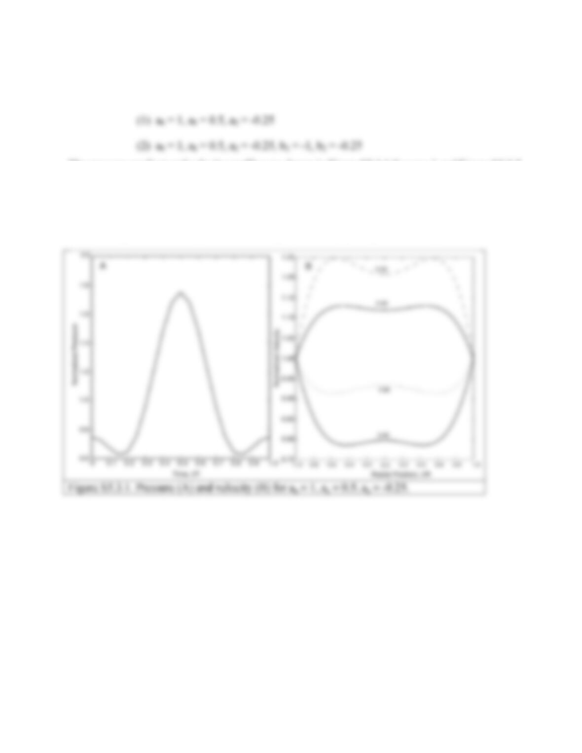
(1) a0 = 1, a1 = 0.5, a2 = -0.25
The pressure gradient and velocity profiles are shown in Figure S5.3.1 for case 1 and Figure S5.3.2
for case 2. Case (1) has positive pressures throughout each cycle. The velocity varies about the
mean value and shapes are similar at all time. Pressure and velocities are symmetric about t/T=0.5.
For case (2) there is a significant negative pressure during the early part of the cycle period causing
fluid deceleration. Fluid accelerates during the pressure upswing and the velocity reaches a
maximum by 0.8. The change in fluid velocity with time lags the pressure change due to inertia.
70
Figure S5.3.2. Pressure (A) and velocity (B) for a0 = 1, a1 = 0.5, a2 = -0.25, b1 = -1, b2 = -0.25.
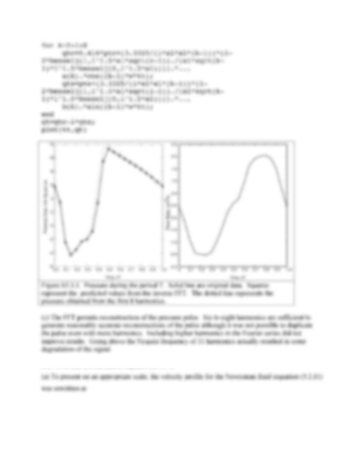
(b) The following program was used to analyze the coronary data in reference [73]. The pressure
gradient as a function of time is shown in Figure S5.3.3. The pressure pulse wave can be well
represented by six to eight harmonics. The pressure is unusual in that it becomes negative during
the early part of the cycle. This is due to vessel compression arising from contraction of the left
ventricle. The flow tracks the pressure, although there is a slight lag. For other results see the paper
by He et al. 1993. Ann. BME 21:45-49.
function transform3(t);
71
for k=2:1:8
5.4. Note that rc is defined in Equation (2.10.7).
(a) To present on an appropriate scale, the velocity profile for the Newtonian fluid (equation (5.2.11)
72
vz= A*R2
i
α
2µ
1 –
Joi3 / 2
α
r / R
( )
Joi3 / 2
α
⎛
⎜
⎜
⎞
⎟
⎟
ei
ω
t
(S5.4.11)
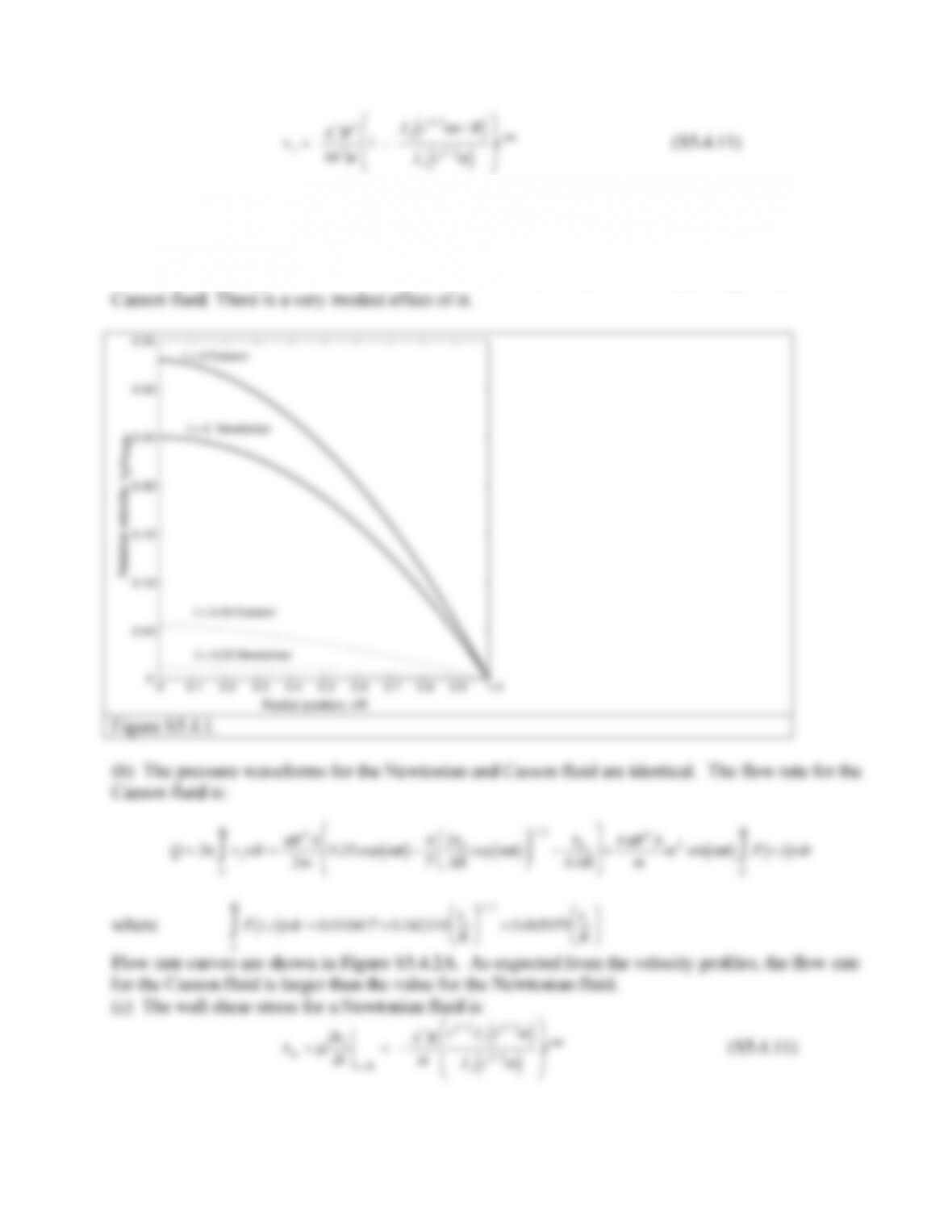
using the definition of α. For presentation purposes, the Casson fluid velocity profile was normalized
by R2A/m and the Newtonian velocity was normalized by R2A*/µ. Shown in Figure S5.4.1 are
results for times of 0.0 s, and 0.50 s. The velocity profiles for the Casson fluid exhibits a slight
amount of flattening. The Newtonian velocities are smaller than the corresponding values for the
Casson fluid. There is a very modest effect of α.
73
For a Casson fluid, the wall shear stress is, using equation (5.11.10):
τ
w =
τ
0
1 / 2 +m
∂
vz
∂
r
⎛
⎝
⎜ ⎞
⎠
⎟
r=R
⎛
⎝
⎜
⎜
⎞
⎠
⎟
⎟
1 / 2
⎛
⎝
⎜
⎜
⎞
⎠
⎟
⎟
2 = RA
4
⎛
⎝
⎜ ⎞
⎠
⎟ r0
R
⎛
⎝
⎜ ⎞
⎠
⎟
1 / 2
+−2exp(i
ω
t) – 42
τ
o
AR2exp(i
ω
t)
⎛
⎝
⎜ ⎞
⎠
⎟
1 / 2
+ 2
τ
o
AR
+8
α
2sin
ω
t
( )
∂
F( r,t)
∂
rr=R
⎛
⎝
⎜
⎜
⎞
⎠
⎟
⎟
1 / 2
⎡
⎣
⎢
⎢
⎤
⎦
⎥
⎥
2
∂
F( r,t)
∂
rr=R
=−1
16R −rc
R
⎛
⎝
⎜ ⎞
⎠
⎟
1 / 2 2
21 −1
6
⎡
⎣
⎢
⎤
⎦
⎥ −rc
18R2=−1
16R −3
14
rc
R
⎛
⎝
⎜ ⎞
⎠
⎟
1 / 2
−rc
18R2
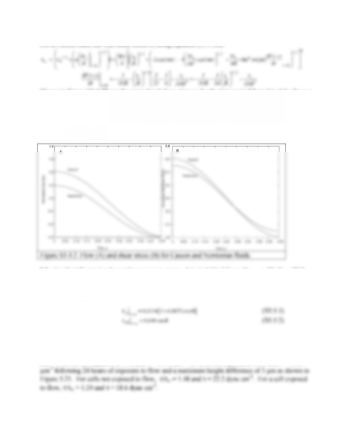
Shown in Figure S5.4.2B are the normalized shear stresses for the time period from 0 to 0.5 s for α =
1.0 and α = 0.5. The shear stress was calculated using the velocity profiles for the Newtonian fluid
(equation (5.2.11)) and the Casson fluid (equation (5.11.10)) and normalized by AR/m. At early
times, the shear stress for the Casson fluid is greater than the value for the Newtonian fluid. This
difference declines as the magnitude of the velocity declines. When flow is negative, the shear stress
for the Casson fluid again becomes slightly greater in magnitude than the value for the Newtonian
fluid.
Figure S5.4.2. Flow (A) and shear stress (B) for Casson and Newtonian fluids.
and a=0.17 cm. The value of δ is 0.082 which may be at the limit of applicability of equations
(5.4.3) and (5.4.4). The average fluid velocity is 7.059 cm s-1. Assume a Newtonian fluid of
viscosity 0.03 g cm-1 s-1. For these data, equations (5.4.3) and (5.4.4) are:
Curvature induces a shear stress component in the θ direction which is as much as 32% of the shear
stress in the z direction. The effect of the curvature on the shear stress in the z direction is modest.
5.6. To solve, use equation (5.7.2) and κ = 0.120 µm-1 for cells not exposed to flow and κ = 0.08
µm-1 following 24 hours of exposure to flow and a maximum height difference of 3 µm as shown in
74
5.7. The net force on the cells is:
F=
τ
dS
∫
(S5.7.1)
This result is derived from the general relation for the surface integral which can be found in
calculus texts.
In order to ensure that the shear stress on a flat surface equals τw, have=0. Integration of (S5.7.1) can
be performed using the function dblquad in MATLAB. The function subroutine is
5.8. The quasi-steady state velocity is Equation (5.2.15)
vzqss =A*R2
4
µ
1−r
R
⎛
⎝
⎜⎞
⎠
⎟
2
⎛
⎝
⎜⎞
⎠
⎟cos(
ω
t)
The flow rate is:
Qqss =2
π
vz
0
R
∫(r,t)rdr =2
π
A*R2
4
µ
0
R
∫1−r
R
⎛
⎝
⎜⎞
⎠
⎟
2
⎛
⎝
⎜⎞
⎠
⎟cos(
ω
t)
⎡
⎣
⎢
⎢
⎤
⎦
⎥
⎥rdr.
Qqss =
π
ΔpR2
2L
µ
cos(
ω
t)R2
2−R2
4
⎛
⎝
⎜⎞
⎠
⎟=
π
ΔpR4
8L
µ
cos(
ω
t)
75
The amplitude is
π
ΔpR4
8L
µ
, the value obtained from the steady flow result.
Q=QQ
5.9. Using the definition of α,
α
=R2
ω
/
ν
and the properties of blood, µ = 0.035 g cm-1 s-1, ρ =
1.05 g cm-3, α = 0.86 for a heart rate of 600 bpm. The amplitude is within 0.8% of the quasi-steady
5.10. (a) Using the definition of power provided,
Solving for Δp:
76
Δp=8µLQ
π
R4
(S5.10.4b)
Replace Q using Equation (S5.10.7b):
77
τ
rz r=R=4µQ
π
R3=4µ
π
R3
π
R3
4
Em
µ
⎛
⎝
⎜⎞
⎠
⎟
1/ 2
⎛
⎜⎞
⎟=µ
Em
( )
1/ 2
(S5.10.10)
5.11. (a) The relationship between the flow rate in the parent vessel and the two daughter vessels is:
78
Solution to Problems in Chapter 6, Section 6.12
6.1. For oxygen, the partial molar volume is 25.6 cm3 mol-1. Application of the Wilkie-Chang
equation (Equation (6.6.25)) results in the following value for the diffusion coefficient, Dij = 2.0 x
6.2. If the measurements for both molecules are assumed to occur at the same temperature and
both can be treated as spheres, then the diffusion coefficients are related by:
D2
D1
= R2
R1
and D2 = 1.7 x 10⁻⁷ cm2 s-1
6.3. (a) For a nonconstant value of δ, Equation (6.5.5.c) is:
1 / 2
Fig S6.3.1
After 500 steps Equation (6.5.6) indicates that the root mean square displacement equals (500)1/2δ or
11.18. Forty two simulations were performed and the root mean square displacement was 11.31 ±
8.31, a 1.16% error (Figure S6.3.2). Thirty three simulations are needed to be within 10% of the
theoretical value.
The relation between the rms displacement and the absolute value of displacement after 500 steps is
linear. The scatter represents the variability arising from the random number generation.
6.4.
Dij = kB
T
f
For a prolate ellipsoid (p=a/b>1)
f =6πµb p2 – 1
( )
1/2
ln p+(p2 – 1)1/2
[ ]
80
For a cylinder of radius a and length L
f ≈ 8πµL
3ln(L / a) – 0.94
6.5. (a) Assume steady state, no reactions, no convection and a dilute solution. A mass balance on
the volume element shown in Figure 6.28 is:
This result indicates that the total number of moles passing through any cross section is constant.
Because the area changes with x, the flux decreases with increasing cross-sectional area.
(b) Integrating the material balance equation:
dCi
1-xi in the expression for the flux is initially 0.9999 and grows. Thus, the flux can be approximated
as:
81
In spherical coordinates, the time to reach steady state is R2/Dij. For the values given the time is 1.25
x 10-4 s. For the problem given this is the time that it would take for the gas to leave the alveolus.
This is much shorter than the time between breathes, 5 sec.
6.7. K = Cm/C. Since the same solvent is on both sides of the membrane, K should be the same on
both sides.
(a) This is feasible and K < 1.
6. 8. For this problem there is a steady state, and one-dimensional diffusion in a dilute solution.
The two regions have cross-sectional areas A1 and A2, respectively. The conservation relations for
each phase are:
6.9. (a) Assume Φ1 = Φ 2 = 1. From Equation (6.6.16b), Deff = 8.45 x 10⁻⁷ cm2 s-1.
(b) If Φ 1 = Φ 2 and D1 =D2 then the concentration is continuous between the two phases and
82
6.10. The steady state mass balances for one dimensional radial diffusion in cylindrical coordinates
are:
Applying the condition at r = R1 that the fluxes are the same yields: Di1A1 = Di2A2. The conditions
that the concentrations are equal at r = R1 yields,
B2=A1ln R1−D1
D2
ln R1
⎛
⎝
⎜
⎜
⎞
⎠
⎟
⎟ +B1
Applying the other two boundary conditions results in the following:
A1=
Di 2 Co−Ci
( )
⎛
⎞
⎛
⎞
A2=
Di1 Co−Ci
( )
⎛
⎞
⎛
⎞
Equation (6.6.36).
The flux in each phase is:
83
Ni2 =−Di2
dCi1
dr =−Di1Di2 Co−Ci
( )
Di1 ln Ro
R1
⎛
⎝
⎜
⎜
⎞
⎠
⎟
⎟ −Di 2 ln Ri
R1
⎛
⎝
⎜
⎜
⎞
⎠
⎟
⎟
1
r
⎛
⎝
⎜ ⎞
⎠
⎟
By comparing each flux expression, with that for a single component medium, the following relation
can be made for the effective diffusion coefficient:
If the thickness of each layer is much less than the inner radius (i.e. R1-Ri <<Ri and Ro-R1<<Ri),
application of Equation (6.6.37) shows that curvature can be neglected and equation 6.6.16b is
recovered.
6.11. When the volumes are unequal, the mass balance on side 1 is
−V1
dC1
dt
= A mDmK
C1 – C2
( )
L
(S6.11.1)
In order to integrate this expression, we need to relate the concentration C1 and C2. This can be done
by noting that once solute leaves side 1 it is either in the membrane or on side 2. Thus, the loss of
solute from side is balanced by the gain of solute in the membrane or side 2.
dC2
dt
= −V
1
V2
dC1
dt
(S6.11.3)
84
Equation (S6.11.5) is a first order ordinary differentiation equation that can be solved with the use of
an integrating factor. Solving Equation (6.11.5) subject to the initial condition that C1 = Co and C2 =
0, yields:
6.12. For diffusion-limited reactions on the cell surface, Equation (6.9.21) applies for which s is the
coated pit radius and b is the distance between coated pits. This distance is 1.825 µm and k– = 0.31 s–
1. What this means is that if measured values of the dissociation constant are less than 0.31 s-1, then
6.13. (a) Assume that adsorption is diffusion-limited. Equation (6.8.29) can be used to predict the
time to cover the surface. Rearranging this equation gives:
2π
(b) If adsorption is irreversible then albumin, since it is the most abundant protein, will rapidly cover
the entire surface. During the time that albumin absorbs, the fibronectin surface concentration only
6. 14. (a) The mass balance is
−Rate of dissolution
of polymer
⎛
⎝
⎜ ⎞
⎠
⎟ = Rate of transport away
from polymer surface
⎛
⎝
⎜ ⎞
⎠
⎟
85
(d) For the data given, the time for the polymer to dissolve is 145 days. Under this condition the
quasi-steady state assumption is valid.
6.15. In this problem there is unsteady, diffusion in the radial direction with no convection or
chemical reactions. Spherical coordinates should be used and the coordinate origin corresponds to
the center of the sphere. The conservation relation is the same as Equation (6.7.48) with Ri = 0. The
initial condition is 0 < r < R
t≤0
C = Co and the boundary condition at r = 0 is
The boundary condition at r = R is:
The transformations for θ’, η and τ yield the following dimensionless conservation relation and
boundary conditions:
The problem is solved using the approach outlined in Equations (6.8.55)-(6.8.57). The solution to
the conservation relation is:
86
Applying the boundary condition at η = 0 yields B = 0 (cf. Equation 6.8.58 and following). θ’
simplifies to:
Asin(λ) exp(−λ2τ)−Aλcos(λ) exp(−λ2τ) = BiAsin(λη)exp(−λ
2τ)
Rearranging this expression results in the following relation for λ:
Applying the orthogonality relation to the initial condition:
1
1
integral on the right hand side is nonzero for m=n. This integral equals 1/2(1-cosλnsinλn /λn). The
coefficients An are thus equal to the following:
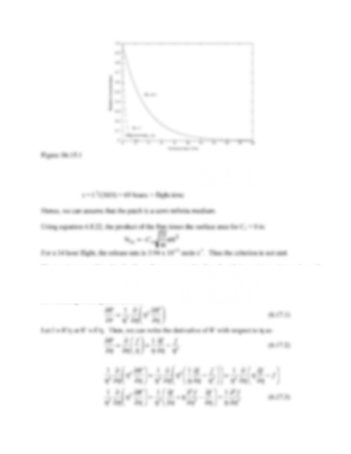
time for its value to reach 0.01 is assumed to be the time to reach steady state.
θ
‘ = 3
θ
‘
η
2d
η
=
∫ 6 sin
λ
n−
λ
ncos
λ
n
( )
2
λ
n
3
λ
n−cos
λ
nsin
λ
n
( )
n =1
∞
∑exp(−
λ
n
2
τ
)
The result is plotted in Figure S6.15.1 for Bi = 0.1, 10 and 1000 which correspond to the range of
parameters given. The dimensionless times to reach steady state are 15 for Bi = 0.1, 0.5 for Bi=10
and 0.4 for Bi=1000. The time increases as the membrane resistance increases relative to diffusion
within the cell (smaller Bi).
87
Figure S6.15.1
6.16. Using Equation (6.8.24), the time period when semi-infinite medium is valid is found by
calculating:
because (1) they do not affect the assumption of a semi-infinite medium (2) they are physical
properties of the patch that can be changed easily.
6.17. Starting with Equation (6.8.53):
∂
θ
‘
∂
τ
=1
η
2
∂
∂
ηη
2∂
θ
‘
∂
η
⎛
⎝
⎜⎞
⎠
⎟
(6.17.1)