181
g1 = x(k)^2;
182
fid = fopen(‘data.txt’, ‘w’);
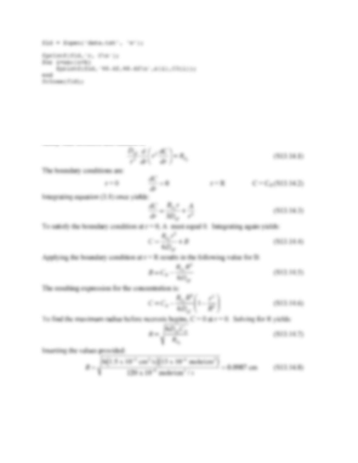
13.14. This is a case of diffusion in spherical coordinates and zero order reaction. To find the
size at which necrosis begins, determine the concentration as a function of radial position. Then
set C to 0 at the center, r = 0 and solve for the radius. At this point oxygen is limiting. Any
tumors bigger than this will have necrosis unless the capillaries penetrate into the tumor. (This
often happens but makes the analysis much more complicated.) The conservation relation for
steady state diffusion and reaction is:
Deff
r2
d
dr r2dC
dr
⎛
⎝
⎜⎞
⎠
⎟=RO2
(S13.14.1)
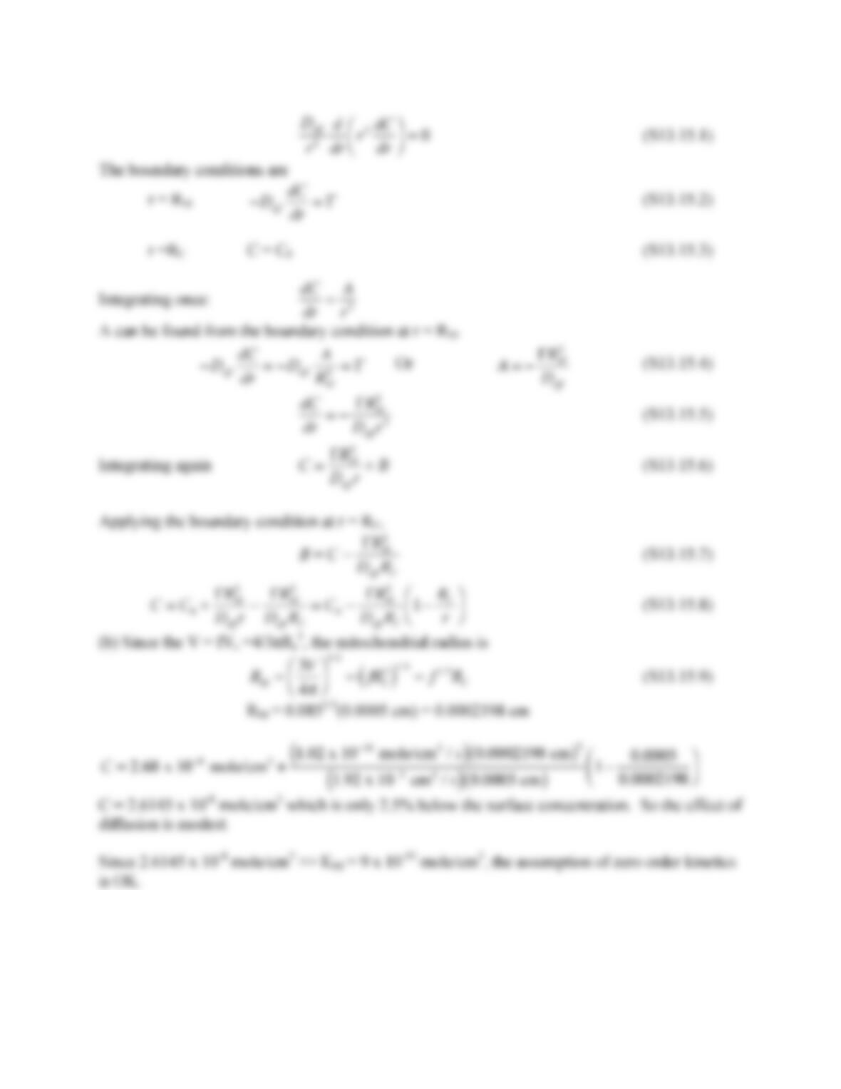
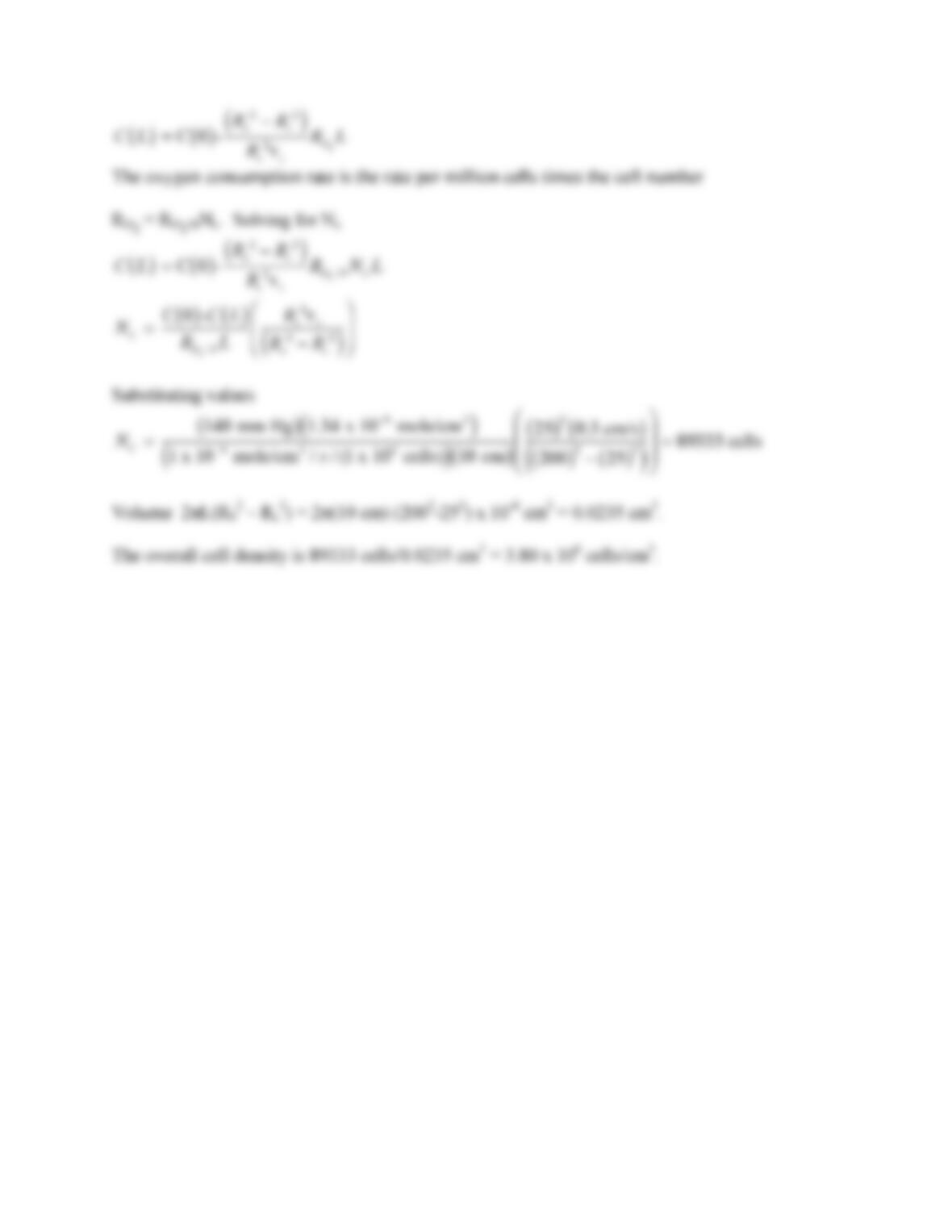
13.15. (a) Since the reaction only occurs on the surface of the mitochondrion, the reaction term
does not appear in the conservation relation and is included in the boundary condition. The
steady state conservation relation in spherical coordinates with no reaction in solution and no
convection is:
183
13.16. Using the Krogh model with axial variation in concentration, equation (13.5.12) applies
from z = 0 to L. The only difference is that the oxygen concentration represents the
concentration in solution.
184
C L
( )
= C 0
( )
–
Ro
2−Rc
2
( )
Rc
2vz
RO2
L
The oxygen consumption rate is the rate per million cells times the cell number
RO2 = RO2/NNc. Solving for Nc
C L
( )
= C 0
( )
–
Ro
2−Rc
2
( )
Rc
2vz
RO2/NNCL
NC = C 0
( )
–C L
( )
RO2/NL
Rc
2vz
Ro
2−Rc
2
( )
⎛
⎝
⎜⎞
⎠
⎟
Substituting values
NC = 140 mm Hg
( )
1.34 x 10⁻⁹ mole/cm3
( )
1 x 10⁻⁹ mole/cm3/s/ (1 x 10⁶ cells)
( )
10 cm
( )
25
( )
20.3 cm/s
( )
200
( )
2−25
( )
2
( )
⎛
⎝
⎜
⎜
⎞
⎠
⎟
⎟=89333 cells
Volume 2πL(R02 – Rc2) = 2π(10 cm) (2002-252) x 10-8 cm2 = 0.0235 cm3.
The overall cell density is 89333 cells/0.0235 cm3 = 3.80 x 10⁶ cells/cm3.
185
Solution to Problems in Chapter 14, Section 14.7
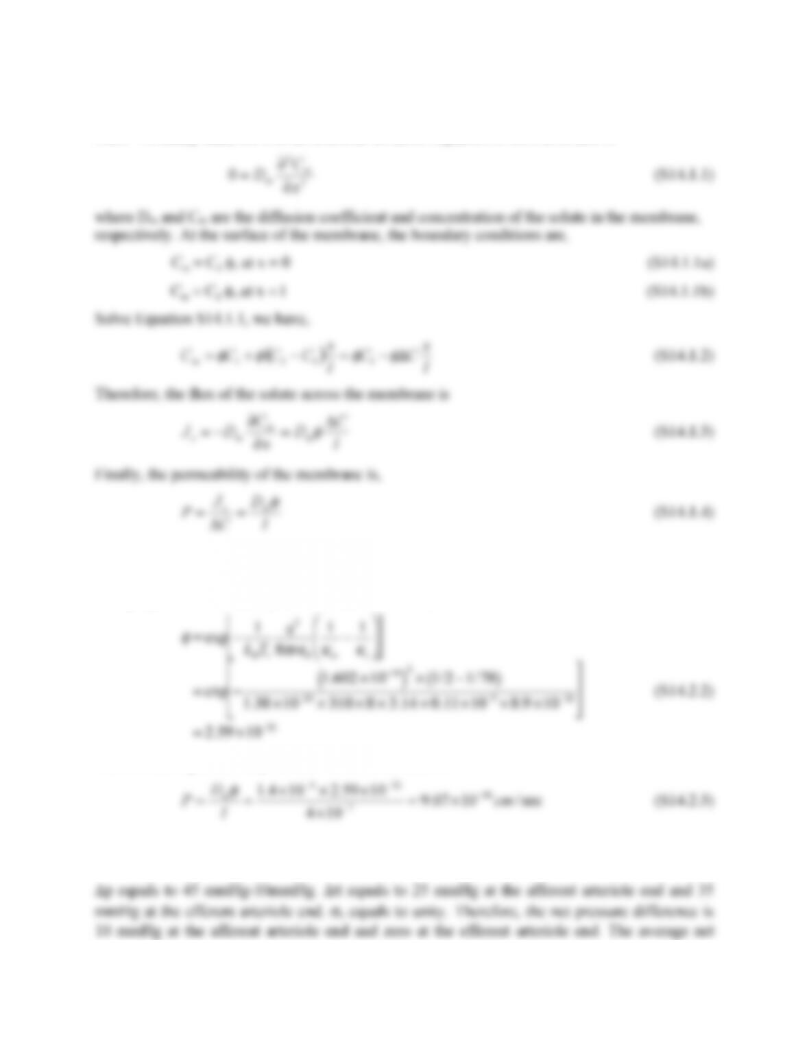
14.1. At steady state, the one-dimensional diffusion equation in the membrane is
2
2
0
x
C
Dm
m∂
∂
=
(S14.1.1)
where Dm and Cm are the diffusion coefficient and concentration of the solute in the membrane,
respectively. At the surface of the membrane, the boundary conditions are,
Cm = C1 φ, at x = 0 (S14.1.1a)
Cm = C2 φ, at x = l (S14.1.1b)
Solve Equation S14.1.1, we have,
( ) l
x
CC
l
x
CCCCmΔ−=−+=
φφφφ
1121
(S14.1.2)
Therefore, the flux of the solute across the membrane is
l
C
D
x
C
DJ
m
m
ms
Δ
=
∂
∂
−=
φ
(S14.1.3)
Finally, the permeability of the membrane is,
l
D
C
J
Pms
φ
=
Δ
=
(S14.1.4)
14.2. The charge of H3O+ is q = 1 × (1.602×10–19 C) = 1.602×10⁻¹⁹ C (S14.2.1)
Using Equation 14.2.5, the partition coefficient of H3O+ in the membrane is
φ
=exp −1
kBTr
q2
8
π
r
ε
0
1
κ
m
−1
κ
s
⎛
⎝
⎜
⎞
⎠
⎟
⎡
⎣
⎢
⎤
⎦
⎥
=exp −1.602 ×10⁻¹⁹
( )
2×1/2 −1/78
( )
1.38 ×10−23 ×310 ×8×3.14 ×0.11×10−9×8.9 ×10−12
⎡
⎣
⎢
⎢
⎤
⎦
⎥
⎥
=2.59 ×10−52
(S14.2.2)
Therefore, the permeability of H3O+ in the membrane is
sec/1007.9
104
1059.2104.1 50
7
524
cm
l
D
Pm−
−
−−
×=
×
×××
==
φ
(S14.2.3)
14.3. The net pressure difference between the blood and the Bowman’s space is
)(
πσ
Δ−Δ s
p
.
Δp equals to 45 mmHg-10mmHg. Δπ equals to 25 mmHg at the afferent arteriole end and 35
186
pressure difference is 5 mmHg since the distribution of net pressure difference is a linear
function of the distance along the glomerular capillary.
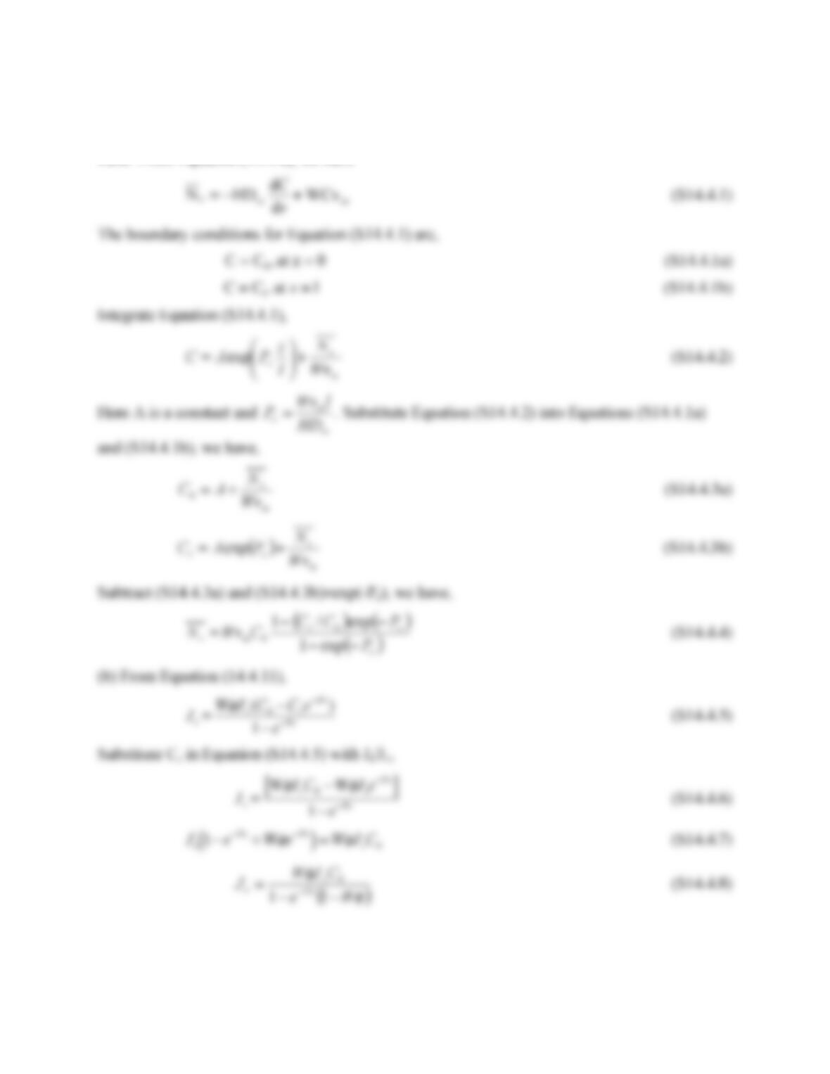
14.4. From Equation (14.4.6), we have
m
sWCv
dz
dC
HDN +−=∞
(S14.4.1)
The boundary conditions for Equation (S14.4.1) are,
C = C0, at z = 0 (S14.4.1a)
C = Cl, at z = l (S14.4.1b)
Integrate Equation (S14.4.1),
m
s
eWv
N
l
z
PAC +
⎟
⎠
⎞
⎜
⎝
⎛
=exp
(S14.4.2)
Here A is a constant and
∞
=
HD
lWv
Pm
e
. Substitute Equation (S14.4.2) into Equations (S14.4.1a)
and (S14.4.1b), we have,
m
s
Wv
N
AC +=
0
(S14.4.3a)
( )
m
s
el Wv
N
PAC += exp
(S14.4.3b)
Subtract (S14.4.3a) and (S14.4.3b)×exp(-Pe), we have,
( ) ( )
( )
e
el
ms P
PCC
CWvN
−−
−−
=exp1
exp/1 0
0
(S14.4.4)
(b) From Equation (14.4.11),
Js=W
φ
Jv(C0−Ce−Pe )
1−e−Pe
(S14.4.5)
Substitute C in Equation (S14.4.5) with Js/Jv,
Js=
W
φ
JvC0−W
φ
Jse−Pe
[ ]
1−e−Pe
(S14.4.6)
Js1−e−Pe +W
φ
e−Pe
( )
=W
φ
JvC0
(S14.4.7)
( )
φ
φ
We
CJW
JPe
v
s−−
=−11
0
(S14.4.8)
187
14.5. The continuity equation and the momentum equations in the x and r directions at steady
state are,
( ) 0
1=
∂
∂
+
∂
∂
r
xrv
rrx
v
(S14.5.1)
⎥
⎦
⎤
⎢
⎣
⎡
∂
∂
+
⎟
⎟
⎠
⎞
⎜
⎜
⎝
⎛
∂
∂
∂
∂
+
∂
∂
−=
⎟
⎟
⎠
⎞
⎜
⎜
⎝
⎛
∂
∂
+
∂
∂
2
2
1
x
v
r
v
r
rrx
p
x
v
v
r
v
vxxx
x
x
r
µρ
(S14.5.2)
( ) ⎥
⎦
⎤
⎢
⎣
⎡
∂
∂
+
⎟
⎟
⎠
⎞
⎜
⎜
⎝
⎛
∂
∂
∂
∂
+
∂
∂
−=
⎟
⎟
⎠
⎞
⎜
⎜
⎝
⎛
∂
∂
+
∂
∂
2
2
1
x
v
rv
rrrr
p
x
v
v
r
v
vr
r
r
x
r
r
µρ
(S14.5.3)
The boundary conditions are,
0=
∂
∂
r
vx
, at r = 0 (S14.5.4)
vx = 0, at r = R (S14.5.5)
vr = vw
=K
lpfluid at wall −˜
p
i
( )
, at r = R (S14.5.6)
Here l is the thickness of the wall. Similar to Example 4.7, we can simplify Equations (S14.5.2)
and (S14.5.3) by examining them in dimensionless form. We assume that the velocity and length
scales are Vx0 and L in x direction, and Vr0 and R in r direction. From Equation (S14.5.1), we
have Vr0<<Vx0, since R<<L. By assuming that the inertial force is negligible and removing all
small terms from Equations (S14.5.2) and (S14.5.3), we have,
⎟
⎟
⎠
⎞
⎜
⎜
⎝
⎛
∂
∂
∂
∂
=
∂
∂
r
v
r
rrx
px
µ
(S14.5.7)
0=
∂
∂
r
p
(S14.5.8)
Equation (S14.5.8) indicated that p is independent of r. Therefore, we can directly integrate
Equation (S14.5.7) and obtain the following expression,
Therefore, the flux in the x direction is,
x
p
8
R
rdr2v
R
1
J
2
R
0x
2
vL ∂
∂
µ
−=π⋅
π
=∫
(S14.5.10)
14.6. Based on Equation (14.5.8b), JiL ≈ CiLJvL. Therefore,
188
If the electric charge is conserved after chemical reactions, then
14.7. The initial concentration after intravenous injection is 100mg/3L. According to Equation
(14.4.2), the filtration rate of inulin is,
14.8. The total rate of PAH excretion from the blood equals to the sum of the rates of filtration
and secretion. Therefore, the mass balance equation is,
pm
pm
p
p
pCK
CT
CGFR
td
Cd
V+
−⋅−=
(S14.8.1)
where the values of GFR, Tm and Km are 125 ml/min, 80 mg/min and 0.07 mg/ml, respectively.
The initial condition of Equation S14.8.1 is,
Cp = 100mg/3000 ml = 0.033 mg/ml at t = 0 (S14.8.1a)
189
Substituting the values of GFR, Tm, Km and Vp into Equation S14.8.1, we have,
⎟
⎟
⎠
⎞
⎜
⎜
⎝
⎛
+
+−=
p
p
p
p
C
C
C
td
Cd
07.0
64.0
24
1
(S14.8.2)
( ) 2471.0
07.0 td
Cd
CC
C
p
pp
p−=
+
+
(S14.8.3)
tdCd
CC p
pp
−=
⎟
⎟
⎠
⎞
⎜
⎜
⎝
⎛+
+
37.2
71.0
6.21
(S14.8.4)
21.6ln Cp+0.71
( )
0.743
[ ]
+2.37ln Cp/0.033
( )
=−t
(S14.8.5)
Letting Cp = Cp0/2 = 0.0167mg/ml in Equation S14.8.5 yields the half life of PAH being
2.12min.
14.9. Assume that the water reabsorption in renal tubules depends on the osmotic pressure
difference of Cl– and HCO3– across the epithelial layer. The rate of water flow across the
epithelial layer is,
Jv=−LPS
σ
sCl −Δ
π
Cl −+
σ
sHCO3
−Δ
π
HCO3
−
( )
(S14.9.1)
where
−
ΔCl
π
and
−
Δ
3
HCO
π
are osmotic pressure difference determined by Cl– and HCO3–,
respectively,
−
sCl
σ
and
−
3
sHCO
σ
are osmotic reflection coefficient of epithelial layer to Cl– and
HCO3–, respectively, and LP is the hydraulic conductivity. Based on Equation (9.3.15),
RT)C(Δ=πΔ
(S14.9.2)
Thus,
Jv=−RTLPS
σ
sCl −ΔCCl −+
σ
sHCO3
−ΔCHCO3
−
( )
(S14.9.3)
Using the concentration data provided in this problem, we obtain,
Jv=−RTLPS
σ
sCl −−
σ
sHCO3
−
( )
⋅20mM
(S14.9.4)
Since the epithelial layer is more permeable to Cl– than HCO3–,
−
sCl
σ
is less than
−
3
sHCO
σ
.
Therefore, Jv > 0, indicating that the direction of the driving force is from the lumen of renal
tubule to the interstitial space and water is reabsorbed.
14.10.
190
z
r
Q
Js
Figure S14.10. 1
In the steady state, the mass balance equation of urea in the renal tubule is
R2CP
zd
Cd
Q0 π⋅⋅−−=
(S14.10.1)
The boundary condition of Equation S14.10.1 is,
C = C0, at z = 0. (S14.10.2)
Solving Equation (S14.10.1) yields
⎟
⎟
⎠
⎞
⎜
⎜
⎝
⎛ π
−=z
Q
RP2
expCC 0
(S14.10.3)
At the end of the renal tubule, the concentration of urea is
⎟
⎟
⎠
⎞
⎜
⎜
⎝
⎛ π
−=
Q
RPL2
expCC 0L
(S14.10.4)
Therefore, the total rate of reabsorption is,
⎟
⎟
⎠
⎞
⎜
⎜
⎝
⎛⎟
⎟
⎠
⎞
⎜
⎜
⎝
⎛ π
−−=−=
Q
RPL2
exp1QCQCQCR 0L0
(S14.10.5)
14.11. If the translocation of uniporter is not the rate-limiting step, we have to consider the
effects of all reactions simultaneous. In this case, two general equilibrium for [SE0] and [SEi]
are,
0][][][]][[ =+−− −− isosooooo SEkSEkSEkESk
(S14.11.1)
0][][][]][[ =−+−−− isosiiiii SEkSEkSEkESk
(S14.11.2)
Similar to that in the textbook, we assume that the total number of uniporters in the plasma
membrane is a constant, ET. In addition, we assume that the total number of uniporters on both
sides of the membrane are time-independent. Therefore, we have two more equations,
Tioio ESESEEE =+++ ][][][][
(S14.11.3)
0][][][][ =−+−−− oEiEosis EkEkSEkSEk
(S14.11.4)
We also assume that [Si] equals to zero. Then from Equation S14.11.2, we can derive,
191
si
os
ikk
SEk
SE
−− +
=][
][
(S14.11.5)
Subtract (S14.11.3)k-E by (S14.11.4), we have,
( ) ( )
[ ]
( ) ⎥
⎦
⎤
⎢
⎣
⎡⎟
⎟
⎠
⎞
⎜
⎜
⎝
⎛
+
−
++−
+
=
−−+−
+
=
−−
−−
−−
−
−−−−
−
][
1
][][
1
][
o
si
sEs
sETE
EE
isEosETE
EE
o
SE
kk
kkk
kkEk
kk
SEkkSEkkEk
kk
E
(S14.11.6)
By substituting (S14.11.5) and (S14.11.6) into (S14.11.1), we have
[ ]
[ ]
02
01
][ SA
SA
SEo+
=
(S14.11.7)
Here A1 and A2 are two constants, which are
( ) ( )
si
sEs
sE
TE
kk
kkk
kk
Ek
A
−−
−−
−
−
+
−
++
=
1
(S14.11.8)
( ) ( ) ( )⎥
⎦
⎤
⎢
⎣
⎡
+
−
+++
⎟
⎟
⎠
⎞
⎜
⎜
⎝
⎛
+
++=
−−
−−
−−
−−
−
−
si
sEso
sEoEE
si
ss
so kk
kkkk
kkkkk
kk
kk
kkA2
(S14.11.9)
The net flux of S into the cell is
[ ] [ ] [ ] [ ]
[ ]
om
o
o
si
ss
si-soss SK
SV
SE
kk
kk
kSE – kSEkJ
+
=
⎟
⎟
⎠
⎞
⎜
⎜
⎝
⎛
+
−==
−−
−max
(S14.11.10)
⎟
⎟
⎠
⎞
⎜
⎜
⎝
⎛
+
−=
−−
−
si
ss
skk
kk
kAV 1max
(S14.11.11)
2
AK m=
(S14.11.12)
14.12. Similar to the analysis in the textbook, we assume that the rate-limiting process in
symport is the translocation of substrates between intracellular and extracellular spaces.
Therefore, the binding between substrates and the symporter is at the equilibrium state. Thus, we
have,
192
Figure S14.12.1.
In addition, we assume that the total number of symporters on both sides of the membrane are
time-independent. Thus,
By solving Equations (S14.12.3), (S14.12.5), (S14.12.6) and (S14.12.7), we can obtain the
expression of the net fluxes of A and S. The above equations are equivalent to the random
reactions with αo and αi equal to unity. Therefore, the net fluxes of A and S are,
[ ] [ ]
⎟
⎟
⎠
⎞
⎜
⎜
⎝
⎛−=
−==
−−
−
S
i
A
i
ii
TC
S
o
A
o
oo
TC
t
iCoCSA
KK
]][S[A
kk
KK
]][S[A
kk
X
T
ASTkASTkJJ
(S14.12.8)
where X is a constant,
⎟
⎟
⎠
⎞
⎜
⎜
⎝
⎛+
⎟
⎟
⎠
⎞
⎜
⎜
⎝
⎛+++
+
⎟
⎟
⎠
⎞
⎜
⎜
⎝
⎛+
⎟
⎟
⎠
⎞
⎜
⎜
⎝
⎛+++= −−
S
o
A
o
oo
CT
S
i
A
i
ii
S
i
i
A
i
i
S
i
A
i
ii
CT
S
o
A
o
oo
S
o
o
A
o
o
KK
]][S[A
kk
KK
]][S[A
K
][S
K
][A
KK
]][S[A
kk
KK
]][S[A
K
][S
K
][A
X
1
1
(S14.12.9)
193
Solution to Problems in Chapter 15, Section 15.6
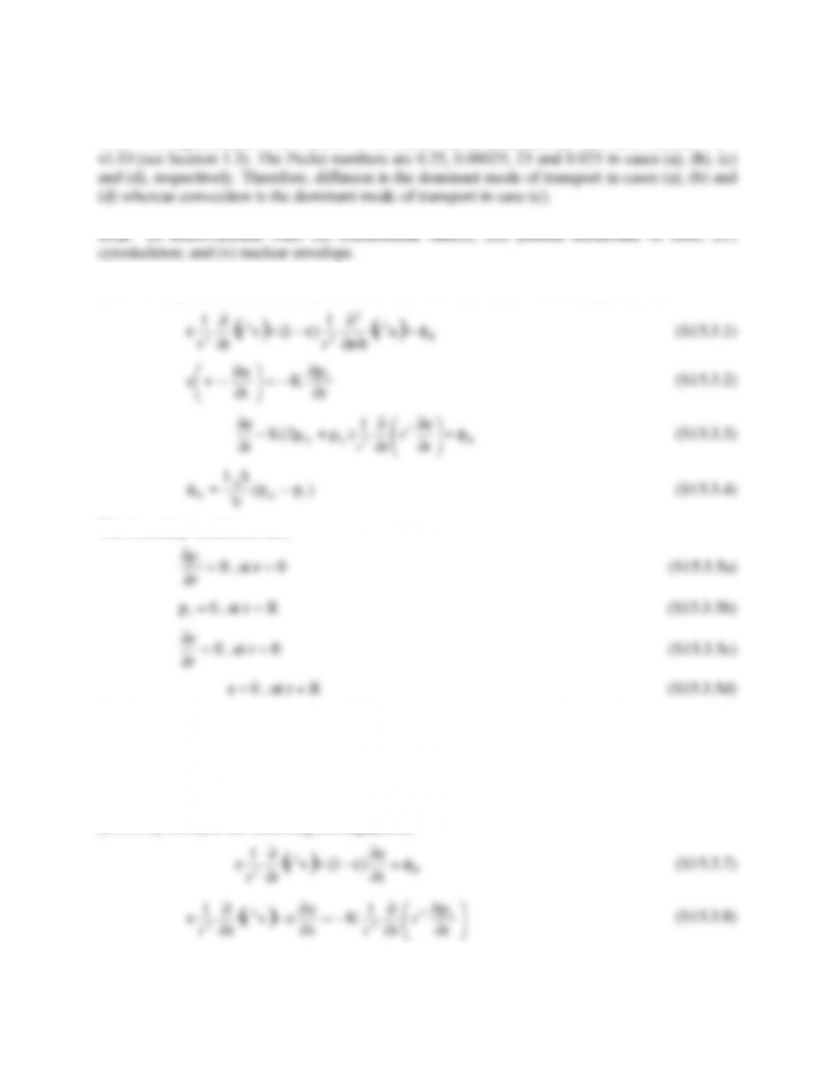
15.1. The significance of convection vs. diffusion can be evaluated by the Peclet number, Pe =
vL/D (see Section 1.3). The Peclet numbers are 0.25, 0.00025, 25 and 0.025 in cases (a), (b), (c)
15.2. (i) microvascular wall; (ii) extracellular matrix; (iii) plasma membrane of cells; (iv)
15.3. In a spherical coordinate system, the mass and momentum balance equations are
( ) ( ) B
2
2
2
2
2ur
tr
r
1
)1(vr
r
r
1φ=
∂∂
∂
ε−+
∂
∂
ε
(S15.3.1)
r
p
K
t
u
vi
∂
∂
−=
⎟
⎠
⎞
⎜
⎝
⎛
∂
∂
−ε
(S15.3.2)
B
2
2
Gr
e
r
r
r
1
)2(K
t
eφ=
⎟
⎠
⎞
⎜
⎝
⎛
∂
∂
∂
∂
µ+µ−
∂
∂
λ
(S15.3.3)
)pp(
V
SL
i1e
p
B−=φ
(S15.3.4)
The boundary conditions are,
∂pi
∂r
=0
, at r = 0 (S15.3.5a)
0pi=
, at r = R (S15.3.5b)
∂e
∂r
=0
, at r = 0 (S15.3.5c)
0e =
, at r = R (S15.3.5d)
Similar to the derivations in Section 15.3.2, we assume ε is a constant. In the spherical system, it
can be written as
Error! Objects cannot be created from editing field codes.
(S15.3.6)
Substituting Equation (S15.3.6) into Equation (S15.3.1) and taking the divergence of Equation
(S15.3.2), we have the following two equations,
( ) B
2
2t
e
)1(vr
r
r
1φ=
∂
∂
ε−+
∂
∂
ε
(S15.3.7)
( ) ⎟
⎠
⎞
⎜
⎝
⎛
∂
∂
∂
∂
−=
∂
∂
ε−
∂
∂
εr
p
r
r
r
1
K
t
e
vr
r
r
1i
2
2
2
2
(S15.3.8)
Subtracting Equation (S15.3.8) from Equation (S15.3.7), we have
194
⎟
⎠
⎞
⎜
⎝
⎛
∂
∂
∂
∂
+φ=
∂
∂
r
p
r
r
r
1
K
t
ei
2
2
B
(S15.3.9)
Substituting Equation (S15.3.9) into Equation (S15.3.3), we have
0
r
e
r
r
r
1
)2(K
r
p
r
r
r
1
K2
2
G
i
2
2=
⎟
⎠
⎞
⎜
⎝
⎛
∂
∂
∂
∂
µ+µ−
⎟
⎟
⎠
⎞
⎜
⎜
⎝
⎛
∂
∂
∂
∂
λ
(S15.3.10)
Rearranging Equation (S15.3.10), we have,
( ) 0e)2(p
r
r
r
r
1
Gi
2
2=
⎟
⎟
⎠
⎞
⎜
⎜
⎝
⎛µ+µ−
∂
∂
∂
∂
λ
(S15.3.11)
Integrating Equation (S15.3.11), we have,
2
1
Gi C
r
C
e)2(p +−=µ+µ−λ
(S15.3.12)
where C1 and C2 are constants. Using the boundary conditions described by Equations (S15.3.5a
through d), we have,
e)2(p Gi λ
µ+µ=
(S15.3.13)
Substituting Equations (S15.3.13) and (S15.3.4) into Equation (S15.3.3), we have,
( )
i1e
p
i
2
2
i
G
pp
V
SL
r
p
r
r
r
1
K
t
p
2
1−=
⎟
⎠
⎞
⎜
⎝
⎛
∂
∂
∂
∂
−
∂
∂
µ+µ λ
(S15.3.14)
Equation (S15.3.14) can be transformed into a homogeneous equation by substituting pi – pe1
with p,
( ) ( )
p2
V
SL
r
p
r
rr
1
2K
t
p
G
p
2
2
Gλλ µ+µ−
⎟
⎠
⎞
⎜
⎝
⎛
∂
∂
∂
∂
µ+µ=
∂
∂
(S15.3.15a)
Accordingly, the boundary conditions become,
0
r
p=
∂
∂
, at r = 0 (S15.3.15b)
1e
pp −=
, at r = R (S15.3.15c)
To solve Equations (S15.3.15a) by using the separation of variables method, we need to make
both the equation and boundary conditions homogeneous. Let p = X(r,t) + f(r), and f(r) satisfies
the following equation and boundary conditions,
f
VK
SL
dr
fd
r
dr
d
r
1
0p
2
2−
⎟
⎠
⎞
⎜
⎝
⎛
=
(S15.3.16a)
0
rd
fd =
, at r = 0 (S15.3.16b)
1e
pf −=
, at r = R (S15.3.16c)
195
Then, Equations (S15.3.15a,b,c) become,
( ) ( )
X2
V
SL
r
X
r
r
r
1
2K
t
X
G
p
2
2
Gλλ µ+µ−
⎟
⎠
⎞
⎜
⎝
⎛
∂
∂
∂
∂
µ+µ=
∂
∂
(S15.3.17a)
0
r
X=
∂
∂
, at r = 0 (S15.3.17b)
0X =
, at r = R (S15.3.17c)
The solution of Equation (15.3.16a) is
)sinh(
R
r
sinh
r
Rp
f1e
α
⎟
⎠
⎞
⎜
⎝
⎛α
−=
(S15.3.18)
where α is
KV
SL
RP
=α
(S15.3.19)
The initial condition of pi is determined by the steady state solution of the equation when pe =
pe0.
)pp(
KV
SL
r
p
r
r
r
1
00ei
p
i
2
2−−
⎟
⎠
⎞
⎜
⎝
⎛
∂
∂
∂
∂
=
(S15.3.20)
According to Equation (15.3.15), the solution of pi at steady state is
⎟
⎟
⎟
⎟
⎠
⎞
⎜
⎜
⎜
⎜
⎝
⎛
α
α
−=
)sinh(
)r
R
sinh(
r
R
1pp 0ei
(S15.3.21)
Therefore, the initial condition of X is,
⎟
⎟
⎟
⎟
⎠
⎞
⎜
⎜
⎜
⎜
⎝
⎛
α
α
−−=
)sinh(
)r
R
sinh(
r
R
1)pp(X 1e0e
, (S15.3.22)
Equation (S15.3.17a) with the initial condition of Equation (S15.3.22) can be solved by using the
separation of variables method. The result is,
( )
tf
1n
2
2
n
0e1e
2
n
e
)n(n
R
r
nsin)1(
r
R)pp(2
X−
∞
=
∑α+ππ
⎟
⎠
⎞
⎜
⎝
⎛π−
−α
=
(S15.3.23)
pi = pe1 + X + f
196
( )
tf
1n
2
2
n
0e1e
2
1e
n
e
)n(n
R
r
nsin)1(
r
R)pp(2
)sinh(
R
r
sinh
r
R
1p −
∞
=
∑α+ππ
⎟
⎠
⎞
⎜
⎝
⎛π−
−α
+
⎥
⎥
⎥
⎤
⎢
⎢
⎢
⎡
α
⎟
⎠
⎞
⎜
⎝
⎛α
−=
(S15.3.24)
15.4. If the initial interstitial fluid pressure at r = 0 is p0, then the microvascular pressure can be
determined by Equation (15.3.15),
197
( ) )e1(
)n(n
R
r
nsin)1(
r
Rp2
)sinh(
R
r
sinh
r
R
1pp tf
1n
2
2
n
0e
2
0ei
n
−
∞
=
−
α+ππ
⎟
⎠
⎞
⎜
⎝
⎛π−
α
+
⎥
⎥
⎥
⎥
⎦
⎤
⎢
⎢
⎢
⎢
⎣
⎡
α
⎟
⎠
⎞
⎜
⎝
⎛α
−=∑
(S15.4.2)
When r → 0,
( ) )e1(
n
)1(
)sinh(
1
p
2pp tf
1n
2
2
n
0
2
0i
n
−
∞
=
−
α+π
−
⎟
⎟
⎠
⎞
⎜
⎜
⎝
⎛
α
α
−
α+= ∑
(S15.4.2)
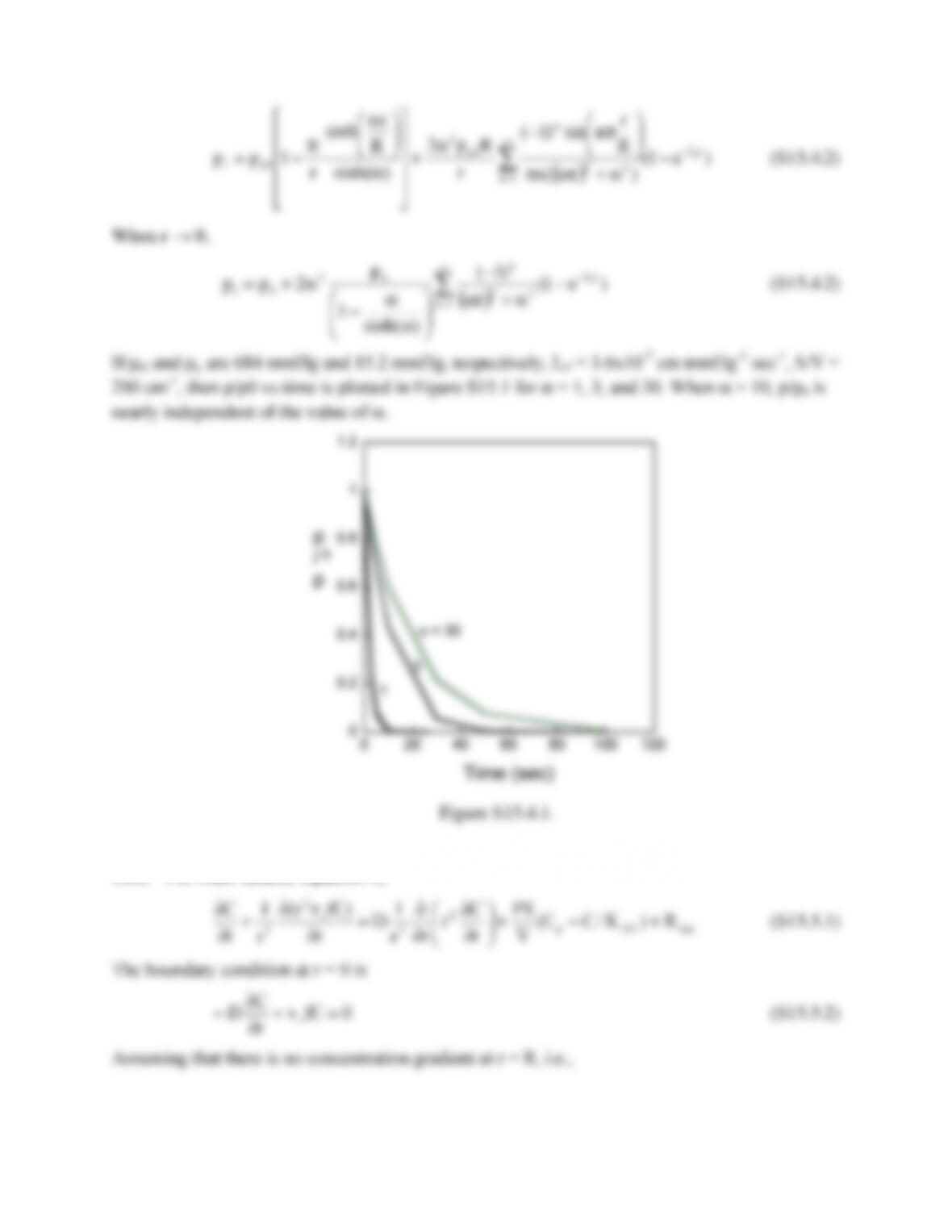
If µG and µλ are 684 mmHg and 15.2 mmHg, respectively, LP = 3.6×10⁻⁷ cm mmHg-1 sec-1, S/V =
200 cm-1, then p/p0 vs time is plotted in Figure S15.1 for α = 1, 3, and 30. When α > 10, p/p0 is
nearly independent of the value of α.
Figure S15.4.1.
15.5. The mass balance equation is,
rxnAVp
2
2
r
2
2R)K/CC(
V
PS
r
C
r
r
r
1
D
r
)fCvr(
r
1
t
C+−+
⎟
⎠
⎞
⎜
⎝
⎛
∂
∂
∂
∂
=
∂
∂
+
∂
∂
(S15.5.1)
The boundary condition at r = 0 is
0fCv
r
C
Dr=+
∂
∂
−
(S15.5.2)
Assuming that there is no concentration gradient at r = R, i.e.,
198
0
r
C=
∂
∂
, at r = R (S15.5.3)
Before the infusion starts, there is no drug in the tumor tissue, i.e.,
C = 0, at t = 0 (S15.5.4)
The velocity profile in the tumor tissue is given by Equation 15.3.16,
⎥
⎦
⎤
⎢
⎣
⎡⎟
⎠
⎞
⎜
⎝
⎛α
−
⎟
⎠
⎞
⎜
⎝
⎛αα
αε
=
R
r
sinh
R
r
cosh
R
r
)sinh(r
RKp
v2
e
r
(S15.5.5)
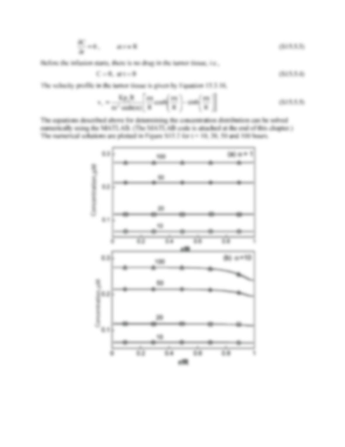
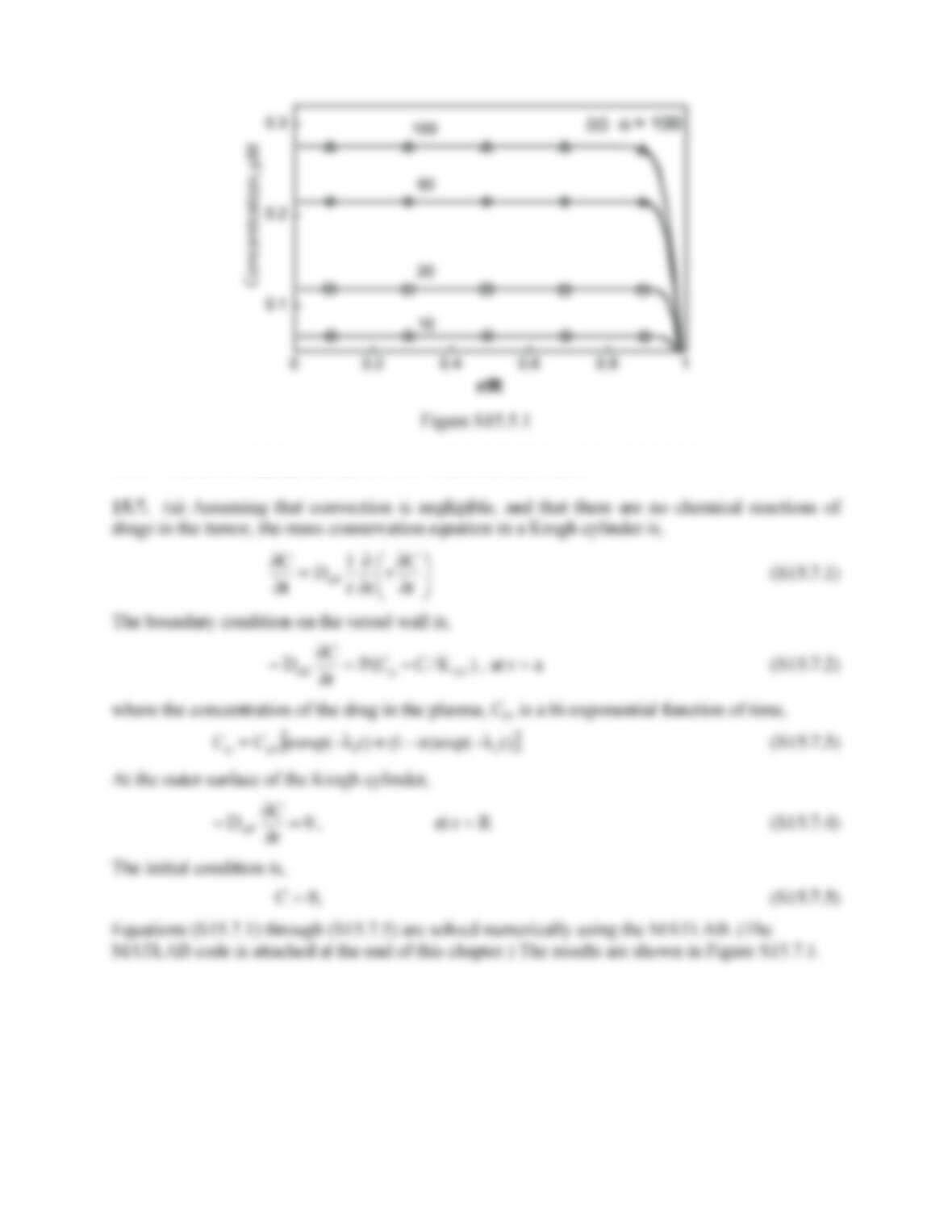
The equations described above for determining the concentration distribution can be solved
numerically using the MATLAB. (The MATLAB code is attached at the end of this chapter.)
The numerical solutions are plotted in Figure S15.2 for t = 10, 20, 50 and 100 hours.
199
Figure S15.5.1
15.6. Statements (a), (c) and (d) are true. Statement (d) is false.
200
Figure S15.7.1.
(b) The dependence of drug distribution on Deff and P can be evaluated, based the MATLAB
(c) The index of spatial nonuniformity (ISN) is defined as
)1N(NC
)CC(
ISN
2
N
1j
−
−
=
∑
=
(S15.7.6)
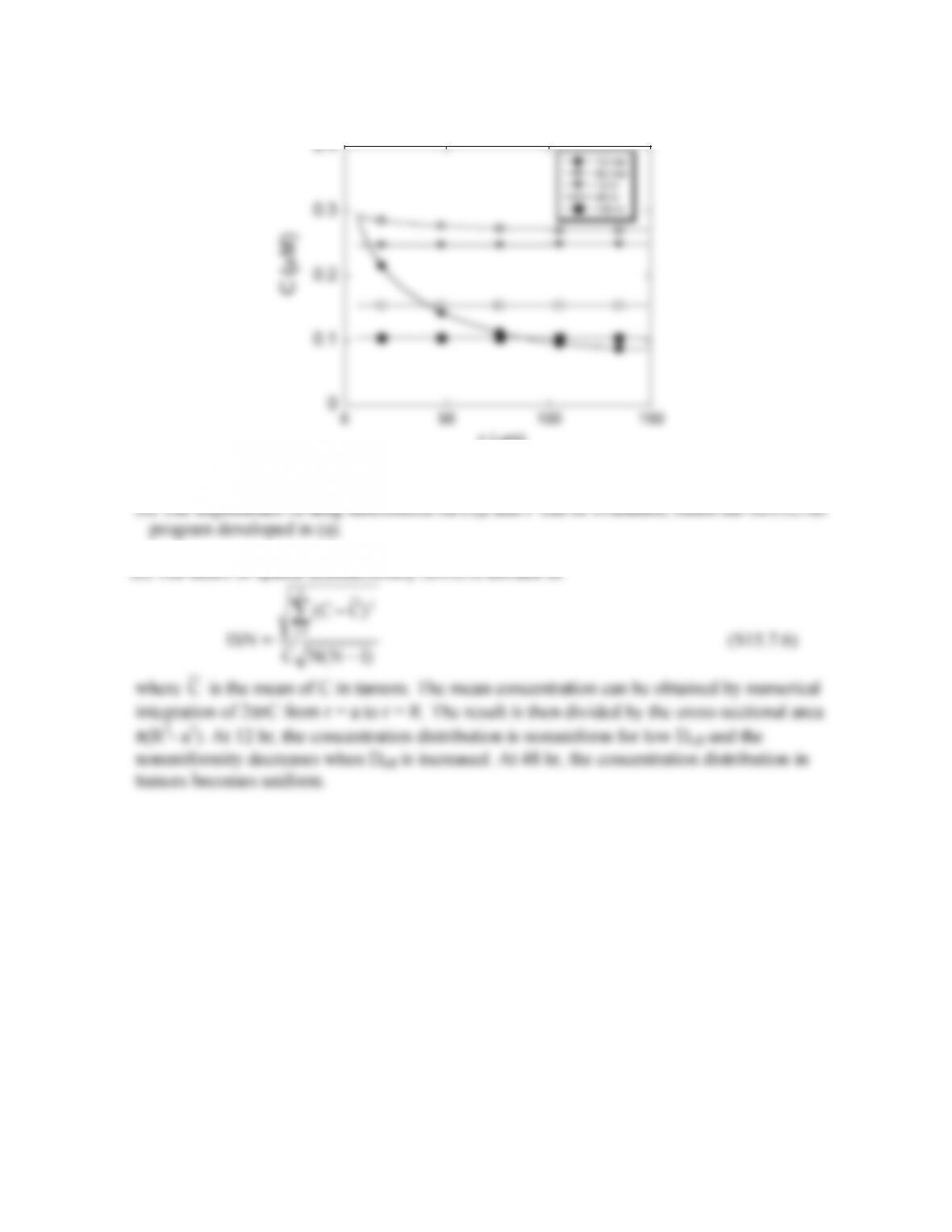
where
C
is the mean of C in tumors. The mean concentration can be obtained by numerical
integration of 2πrC from r = a to r = R. The result is then divided by the cross-sectional area
π(R2– a2). At 12 hr, the concentration distribution is nonuniform for low Deff and the
nonuniformity decreases when Deff is increased. At 48 hr, the concentration distribution in
tumors becomes uniform.
0
0.1
0.2
0.3
0.4
0 50 100 150
10 min
60 min
12 hr
48 hr
100 hr
r (µm)