41
τ
z
θ
z=0=
µ∂
v
θ
∂
zz=0
=
µω
α
1−0.003294
ε
2
⎡
⎣⎤
⎦
(S3.12.11)
3.13. Equation (3.6.32) is:
dUo
Let u = vt –Uo. Thus, d = -du. As a result, equation (3.6.32) becomes
du
dt
= – 9µ
2
ρ
pR2u
3.14. For an adherent leukocyte, H/R = 1 and F*(H/R) = 1.69. Thus, the drag force is
3.15. This problem is the inverse of the example discussed in Section 3.6.2. That is, the fluid far
from the sphere has a zero velocity and the sphere is moving at a constant speed U0.
To find the pressure field, substitute equations (3.3.8a,b) into equations (3.6.7a,b) and compute the
derivatives. These derivatives are:
42
1
r2sin
θ
∂
∂θ
sin
θ∂
vr
∂θ
⎛
⎝
⎜ ⎞
⎠
⎟ =−Uocos
θ
3R
r3−R3
r5
⎛
⎝
⎜
⎞
⎠
⎟
∂
vr
∂
r
=Uo
2
cos
θ
d
dr
3R
r−R3
r3
⎛
⎝
⎜
⎞
⎠
⎟ =Uo
2
cos
θ
−3R
r2+3R 3
r4
⎛
⎝
⎜
⎞
⎠
⎟
1
r2
∂
∂
r
r2
∂
vr
∂
r
⎛
⎝
⎜ ⎞
⎠
⎟ =3Uo
2r 2cos
θ∂
∂
r−R+R3
r2
⎛
⎝
⎜
⎞
⎠
⎟ =−3Uo
R3
r5
⎛
⎝
⎜
⎞
⎠
⎟ cos
θ
∂
v
θ
∂
r
=3Uo
4
sin
θ
R3
r4+R
r2
⎛
⎝
⎜
⎞
⎠
⎟
1
r2
∂
∂
r
r2
∂
v
θ
∂
r
⎛
⎝
⎜ ⎞
⎠
⎟ =3Uo
4
sin
θ
1
r2
∂
∂
r
R3
r2+R
⎛
⎝
⎜
⎞
⎠
⎟ =−3Uo
2
R3
r5
⎛
⎝
⎜
⎞
⎠
⎟ sin
θ
∂
v
θ
∂θ
=−Uo
2
cos
θ
R
r
⎛
⎝
⎜⎞
⎠
⎟
3
+3R
r
⎛
⎝
⎜⎞
⎠
⎟
1
r2sin
θ
∂
∂θ
sin
θ∂
v
θ
∂θ
⎛
⎝
⎜⎞
⎠
⎟=−Uo
4 sin
θ
R3
r5+3R
r3
⎛
⎝
⎜⎞
⎠
⎟
∂
∂θ
sin
θ
cos
θ
( )
1
r2sin
θ
∂
∂θ
sin
θ∂
v
θ
∂θ
⎛
⎝
⎜⎞
⎠
⎟=4
Uocos2
θ
−sin2
θ
( )
2 sin
θ
R3
r5+3R
r3
⎛
⎝
⎜⎞
⎠
⎟=−Uo1−2 sin2
θ
( )
4 sin
θ
R3
r5+3R
r3
⎛
⎝
⎜⎞
⎠
⎟
2
r2
∂
vr
∂θ
=−Uosin
θ
3R
r3−R3
r5
⎛
⎝
⎜
⎞
⎠
⎟
Equation (3.6.7a) becomes
0=−
∂
p
∂
r+
µ
Uocos
θ
−3R3
r5−3R
r3−R3
r5
⎛
⎝
⎜
⎞
⎠
⎟ −3R
r3−R3
r5
⎛
⎝
⎜
⎞
⎠
⎟ +1
2
R3
r5+3R
r3
⎛
⎝
⎜
⎞
⎠
⎟ +1
2
R3
r5+3R
r3
⎛
⎝
⎜
⎞
⎠
⎟
⎡
⎣
⎢
⎤
⎦
⎥
Simplifying
0=−
∂
p
∂
r+
µ
Uocos
θ
−3R3
r5−23R
r3−R3
r5
⎛
⎝
⎜
⎞
⎠
⎟ +R3
r5+3R
r3
⎛
⎝
⎜
⎞
⎠
⎟
⎡
⎣
⎢
⎤
⎦
⎥ =−
∂
p
∂
r−
µ
Uocos
θ
3R
r3
⎛
⎝
⎜ ⎞
⎠
⎟
(S3.15.1)
Likewise, after substituting into Equation (3.6.7b), we have
0=−1
r
∂
p
∂θ
+
µ
Uosin
θ
−3
2
R3
r5
⎛
⎝
⎜
⎞
⎠
⎟ +1
2
R3
r5+3R
r3
⎛
⎝
⎜
⎞
⎠
⎟ −3R
r3−R3
r5
⎛
⎝
⎜
⎞
⎠
⎟
⎡
⎣
⎢
⎢
⎤
⎦
⎥
⎥
This result simplifies to:
0=−1
r
∂
p
∂θ
−
µ
Uosin
θ
3R
2r3
⎛
⎝
⎜ ⎞
⎠
⎟
(S3.15.2)
Integrating Equation (S3.15.1) yields
p=C1+
µ
Uocos
θ
3R
2r2
⎛
⎝
⎜ ⎞
⎠
⎟
43
As r → ∞, p approaches p∞ which is the value of C1.
44
The magnitude of the drag force is identical to the value obtained for the case of a stationary sphere
exposed to a uniform velocity U0. The minus sign indicates that the drag force is in the direction
opposite the motion of the sphere.
3.16. (a) The Reynolds number for the cell at y = 0 is Re = ρ<v>Dleukocyte/µ. The velocity can be
obtained from the definition of the wall shear stress and equation 2.7.24.
(b) State force balances in the x- and y-directions acting on the cell. Neglect acceleration of the cell.
x direction Force of the fluid on the cell = Drag force
(c) Solve the force balances to determine the distance traveled by a cell which is initially at the
centerline.
To determine the distance traveled, we need to compute the change in x and y position. The cell
velocity in the x direction is just the change in x position with time. Likewise, the cell velocity in the
y direction is just the change in y position with time. The fluid velocity is given by equation 2.7.24.
Thus, the force balances are rewritten as:
x direction
dx
dt
=3
2v1−4y2
h2
⎛
⎝
⎜
⎞
⎠
⎟
Where vt is the terminal velocity defined by equation 3.6.30. Notice that the displacement of the cell
in the x direction depends upon the vertical position of the cell. From the force balance in the y
direction, we have, y=vtt, assuming that the cell was motionless prior to t = 0. Thus, the y location of
the cell is now known as a function of time. The force balance in the x direction becomes
dx
dt
=3
2
v1−4vt
2t2
h2
⎛
⎝
⎜
⎞
⎠
⎟
Integrating with respect to time and starting at x = 0, yields:
x=3
2
v t −4vt
2t3
3h2
⎛
⎝
⎜
⎞
⎠
⎟
45
xo=3
2
v−h
2vt
−
4vt
2−h
2vt
⎛
⎝
⎜
⎞
⎠
⎟
3
3h2
⎛
⎝
⎜
⎜
⎜
⎜
⎞
⎠
⎟
⎟
⎟
⎟
=3
2
hv
vt
−1
2
+1
6
⎛
⎝
⎜ ⎞
⎠
⎟ =−1
2
hv
vt
For the data given, vt = -0.0199 cm s-1 and xo is 12.30h = 0.3074 cm.
(d) This result means that if you measured the number of adherent or rolling cells within 0.30 cm
from the introduction of the cells you would underestimate the true frequency because not all of the
cells have settled to the surface.
3.17. (a) In order to determine the height, we need to know the viscosity, channel width, flow rate
and either the pressure drop or shear stress. From 1, w = 20h, Q per channel is specified in 2 and 3:
Q = (10 cm3/hour)(1 hour/3600 s)/(20 channels) = 1. 39 x 10-4 cm3/s
From statement 5, the shear stress is specified. From equation (2.7.30) we have
τ
yx =−Δp
Lyy=−h/ 2 =Δph
2L
The pressure drop per until length is
Δp
L
=
2
τ
yx
h
Replacing the pressure drop per unit length and w = 20h
Q=
2
τ
yxwh3
12µh
=
τ
yxwh2
6µ
=
20
τ
yxh3
6µ
=
10
τ
yxh3
3µ
(b) The total pressure drop per channel is
Δp=2
τ
yx L
h=2 1
( )
6
0.0069 =952 dyne/cm2
46
The total pressure drop is 20 times this value or 19,049 dyne = 1905 Pa. Thus, the criterion is met.
The Reynolds number is
Re =
ρ
vDh
µ=
ρ
Q2wh
whµ w +h
( )
=2
ρ
Q
µ w +h
( )
Re =0.131
Thus, the flow is laminar and close to the criterion for Stokes flow (Re = 0.1).
3.18. For steady, fully developed laminar flow in a cylindrical tube using rectangular coordinates,
flow is in the z direction and normal to the x-y plane. For fully developed flow, vz =f(x,y) only. All
other velocity components are zero (vx = vy = 0). For steady flow
∂vz
∂t
=0
. (S3.18.1)
Assuming that the channel is horizontal, the Navier-Stokes equation reduces to:
From Equations (S3.18.2a,b), p(z) only. Since p(z) and vz(x,y), each side of Equation (S3.18.2c)
must equal a constant. The constant is equal to –Δp/L, the pressure drop per unit length.
integration. At x2 + y2 = R2, we find that A = -B. This equation already satisfies the condition at x
= 0 and y = 0.
(c) Substituting the expression for vz into Equation (S3.18.3):
The velocity profile is:
47
vz=Δp
4µL R2−x2−y2
( )
=ΔpR2
4µL
1−x2+y2
R2
⎛
⎝
⎜⎞
⎠
⎟
(S3.18.4)
Note: an alternate solution is: vz(x,y) =A+B(x2+y2) C x2y2. This solution does satisfy the boundary
conditions. Using this in Equation (S3.18.3) yields
−Δp
L=
µ
4B+2C x2+y2
( )
( )
(S3.18.5)
In order for the right hand side to equal a constant C must equal 0.
3.19. The solution for an elliptical tube can be obtained by a variation on the approach used in
Problem 3.18. Equation (S.318.3) applies. The boundary condition at x = 0 and y = 0 is unchanged.
The tube surface is given by:
x2
a2+y2
b2=1
(S3.19.1)
Along this surface, vz = 0.
Since this equation and boundary conditions are similar to the flow in a cylindrical tube solved using
rectangular coordinates, we postulate that the solution of the form:
Applying the no slip condition along the ellipse surface, A = -B.
vz=Bx2
a2+y2
b2−1
⎛
⎝
⎜⎞
⎠
⎟
(S3.19.2)
Using this velocity field and taking the second derivatives with respect to x and y,
Solving for B:
B=−Δp
2µL
a2b2
a2+b2
⎛
⎝
⎜⎞
⎠
⎟
(S3,19,4)
Solution to Problems in Chapter 4, Section 4.10
4.1. Begin with equation (4.2.2) for the case of a control volume that changes with time:
Applying Leibniz’s rule (Equation (A.1.29) to the term
∂
∂t
ρ
V ( t )
∫dV
⎛
⎝
⎜
⎞
⎠
⎟
∂
∂t
ρ
V(t)
∫dV
⎛
⎝
⎜
⎞
⎠
⎟ =∂
ρ
∂t
V(t)
∫dV +
ρ
l2
( )
dA ∂l2
( )
∂t−
ρ
l
1
( )
dA ∂l
1
( )
∂t
(S4.1.2a)
where l2 and l1 are the limits of integration of the volume. Since integration is over the entire surface,
the second and third terms on the right hand side of equation (S4.1.2a) represent the sum and
(S4.1.2a) becomes
Applying the divergence theorem to the second term on the right hand side of (S4.1.3)
∂
∂t
ρ
∫dV
⎛
⎜
⎞
⎟ =∂
ρ
∂t
∫dV +
ρ
n•vSdV
∫
(S4.1.4)
where vs is the velocity of the control volume surface (Deen, W.M., Analysis of Transport
Phenomena. 1998, New York: Oxford University Press.). Rearranging and replacing
∂
ρ
∂t
V ( t )
∫dV
in
Equation (S4.1.1)
∂
ρ
∂t
V ( t )
∫dV =∂
∂t
ρ
V ( t )
∫dV
⎛
⎝
⎜
⎞
⎠
⎟ −
ρ
n•vSdV
S
∫=–∇•
ρ
v
( )
dV
V(t)
∫
(S4.1.5)
Replacing the right hand side of Equation (S4.1.5) with Equation (4.2.4) and noting that
ρ
V ( t )
∫dV =m
dm
dt =–
ρ
v – vS
( )
•ndS
∫
(S4.1.6)
49
Further progress can be made if the control volume is applied to a region over which fully developed
flow is established as shown in the figure below.
With these simplifications, the analysis uses the same development presented in Example 4.2. The
control volume can be divided into three regions, 1, 2 and 3. Mass enters through region 1 and exits
through region 3. There is no flow across the walls of the vessel, region 2. The average velocity in
the inlet and outlet can be related by the conservation of mass.
v1
π
R1
2=v2
π
R2
2=v2
π
E2R1
2
(S4.2.2)
velocity at location 1 and E:
Since there is no flow across the surface 3 and flow across surfaces 1 and 2 is in the z direction the
only non-zero component of equation (S4.2.1) is in the z-direction. The z component of the left
hand side of equation (S4.2.1) becomes:
R1
2
2
R2
2
The shear stress is zero over surfaces 1 and 2 and the pressure is zero over surface 3. Because the
detailed velocity field through the taper is not known, the shear stress cannot be computed.
The right hand side of Equation (S4.2.5) represents the net force acting in the z-direction. The force
depends strongly on the taper ratio E. The net pressure force acting on the fluid is obtained by
rearranging equation (S4.2.5)
The pressure drop is increased above the value for flow in a straight tube due to convective
acceleration through the taper and the shear stress acting on the walls of the vessel.
50
4.3. For steady, laminar flow through the entrance region of a cylindrical tube that is horizontally so
that gravity is negligible, the integral form of the conservation of linear momentum, eEquation
(4.3.8), is:
Neglecting gravity, the pressure at r = R is uniform so the integral of pressure over the control
volume surface equals ez(p0 – pLe)πR2 where Le is the entrance length. The integral of the shear
stress represents the net drag force acting on the fluid. Thus, the drag force equals:
The drag force is less than the value in fully developed flow because the flow develops in this region
and the velocity gradients are not as steep.
4.4. From equations (4.3.11d) and (4.3.11e) for the z and r components of the net force on the
branching vessel:
2
ρ
R1
⎝
⎜
⎠
⎟
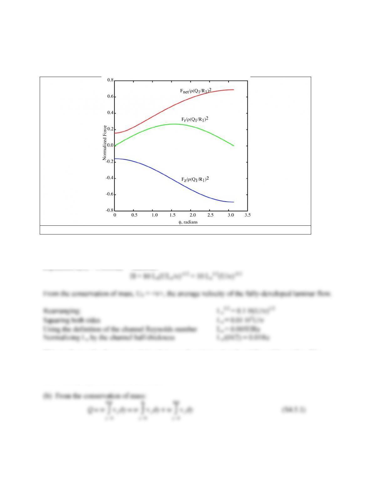
51
The net force is simply Fnet = (Fz2+Fr2)1/2. The results are presented in Figure S4.3.1. The net force
is smallest at an angle of zero degrees. The net force at zero degrees is not zero because the cross-
sectional areas in sections 4 and 5 are greater than 1, resulting in a decrease in velocity through the
tubes. As the branch angle increases, the net force increases, reaching a maximum at 180 degrees.
Figure S4.3.1
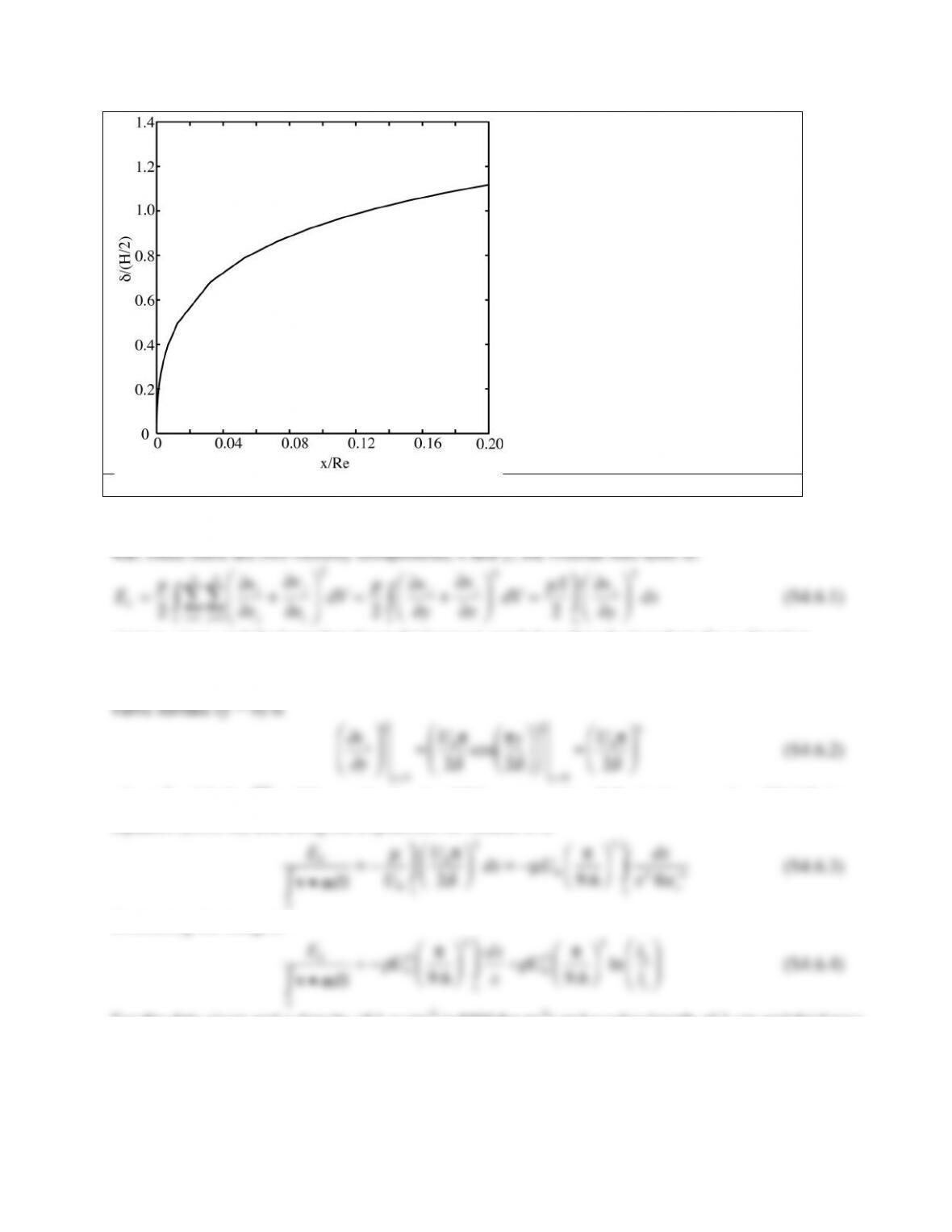
4.5. (a) Let δ = H/2 and x = Le, the entrance length. Rex=Le = ULe/ν. Thus, the boundary layer
expression δ(x) = 5.00xRex-1/2 becomes
H = 10 Le(ULe/ν)-1/2 = 10 Le1/2(U/ν)–1/2
coefficient is the correct magnitude, but is smaller than the measured values. The reasons for this
discrepancy are that the centerline velocity increases as the fluid decelerates near the surfaces and
the boundary layer thickness is not small.
52
Q=wUy
δ
dy
δ
∫+w U( x)dy
H/2
∫=wU
δ
2
+wU( x ) H
2−
δ
⎛
⎝
⎜ ⎞
⎠
⎟ =wU( x ) H
2−
δ
2
⎛
⎝
⎜ ⎞
⎠
⎟
(S4.5.2)
53
Figure S4.5.1
4.6. Since there are two velocity components, x and y, the viscous loss term is:
2
since vy << vx and the boundary layer thickness is much less than the length in the x direction.
The velocity gradient can be estimated assuming that viscous stresses arise in a thin boundary layer
near the valve surface. If the velocity is vx = U0sin(πy/2δ), then the square of velocity gradient at the
valve surface (y = 0) is
2
2
where δ = 4.8xRex-1/2 and Rex = ρU0x/µ. In addition, <v> = U0. Substituting equation (S4.6.2) into
equation (S4.6.1c) and using the expression for results in δ.
EV
v•n
S
∫dS =−
µ
U0
U0π
2
δ
⎛
⎝
⎜⎞
⎠
⎟
2
dx
l1
l2
∫=−µU0
π
9.6
⎛
⎝
⎜⎞
⎠
⎟
2dx
x2Rex
−1
l1
l2
∫
(S4.6.3)
Evaluating the integral:
EV
v•n
S
∫dS
=−
ρ
U0
2π
9.6
⎛
⎝
⎜⎞
⎠
⎟
2dx
x
=
l1
l2
∫
ρ
U0
2π
9.6
⎛
⎝
⎜⎞
⎠
⎟
2
ln l2
l1
⎛
⎝
⎜⎞
⎠
⎟
(S4.6.4)
For the data given and a density of 1 g cm-3 (=1000 kg m-3) and a valve length of 1 cm and thickness
0.1 cm, l2/l1 = 1/0.9=1.1. EV = -0.408 N m-2. This corresponds to 0.0075 mm Hg. The viscous
losses are much smaller than the pressure drops induced by convective acceleration.
54
Note that this analysis is quite simplified. A more thorough analysis would include the effect of
viscous losses due to the jet as discussed in [11].
4.7. Setting v2 = vmax in equation (4.4.18), the relative error in neglecting v1 is
error =vmax
2−v1
2
vmax
2=1−v1
2
vmax
2≥0.90
Solving for v1,
4.8. From equation (4.4.18) p1 – p2 = (4 s2m-2 mm Hg)(1.32-0.52) m2s-2 = 5.76 mm Hg
The cross-sectional area of the valve can be determined by a mass balance
v1ARV = v2Avalve
4.9. This problem is similar to the previous except that the atrial area must be calculated from the
diameter.
4.10 First calculate the Reynolds number treating blood as a Newtonian fluid. Thus, from Table
2.5, ρ = 1.05 g cm-3 , µ = 0.03 g cm–1 s-1 and ν = 0.0286 cm2 s-1.