Solution to Problems in Chapter 17, Section 17.10
17.1. In words, the conservation relation is:
#
&
#
&
#
&
#
&
Energy of Rate
Workof Rate
Energy of RateNet
Energy of Rate
17.2. The work is:
W=Findx
!=Fdx
!
since the force and unit outward normal are
both positive. Normally, a protein is present in a specific conformation which is much
less than the maximum length, know as the contour length, L. The contour length is the
length of the polymer if each chain element were aligned along a line.
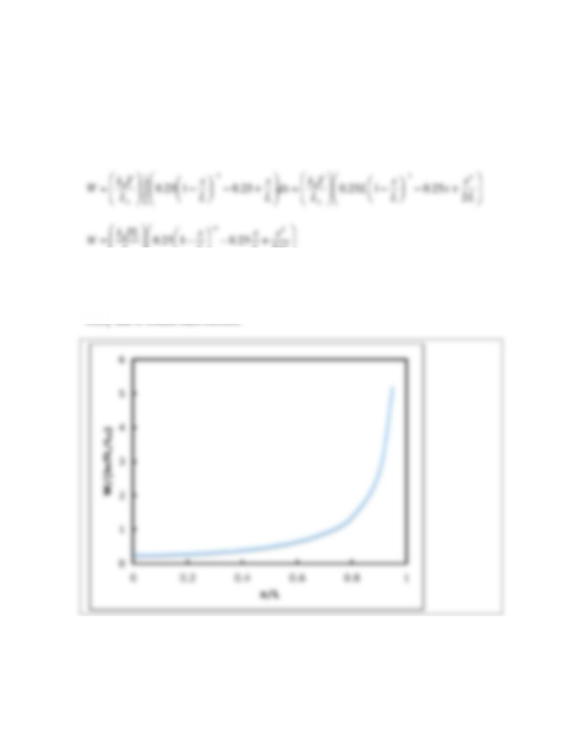
Substituting for the wormlike chain model:
‘2
x
‘1
229
17.3. Note: The equation listed in the problem statement should be:
!
!v=
“
:#v=
µ
dvz
dr
$
%
&‘
(
)
2
The shear stress tensor for a Newtonian fluid is:
!
=
µ
“v+“v
( )
T
( )
(S17.3.1)
!
!v=
“
:#v=
µ
#v+#v
( )
( )
:#v
(S17.3.2)
Using the summation convention for vectors and tensors
µ
!v+!v
( )
T
( )
:!v=
µ
“vi
“xj
+“vj
“xi
#
$
%&
‘
(eiej
j=1
3
)
i=1
3
)
#
$
%&
‘
(:“vk
“xl
ekel
l=1
3
)
k=1
3
)
#
$
%&
‘
(
(S17.3.3)
Since
eiej:ekel=ejiek
( )
eiiel
( )
=
!
jk
!
il
, Equation (S17.3.3) becomes:
µ
!v+!v
( )
T
( )
:!v=
µ
“vi
“xj
#
$
%&
‘
(“vj
“xi
#
$
%&
‘
(+“vj
“xi
#
$
%&
‘
(
2
#
$
%&
‘
(
j=1
3
)
i=1
3
)
(S17.3.4)
For fully developed steady, laminar flow in a cylindrical tube of radius R,
!
=
µ
“vz
“r+“vr
“z
#
$
%&
‘
(erez
Using the symmetry property of the shear stress, τij = τji:
!
!v=
µ
“vz
“r
erez+“vr
“z
ezer
#
$
%&
‘
(:“vz
“r
erez
=
µ
“vz
“r
erez+“vz
“r
ezer
#
$
%&
‘
(:“vz
“r
erez=
µ
“vz
“r
“vz
“r
#
$
%&
‘
(=
µ
“vz
“r
#
$
%&
‘
(
2
(S17.3.5)
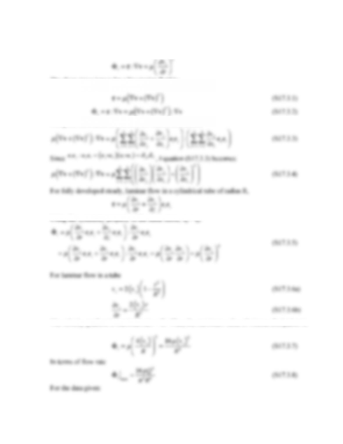
For laminar flow in a tube
vz=2 vz1!r2
R2
“
#
$%
&
‘
(S17.3.6a)
!vz
!r
=
2 vzr
R2
(S17.3.6b)
The velocity gradient is maximum at r = R. Thus, the maximum value of viscous dissipation is:
2
2
230
2
radial conduction with viscous dissipation. From Equations (17.2.8), (17.2.9), (17.2.12) and
(S17.3.6b), the following result is obtained.
k
r
d
dr rdT
dr
!
“
#$
%
&=‘!
(v=‘16 µQ2r2
)
2R8
(S17.3.9)
The boundary conditions are that for r = 0, the flux is zero and at r = R, T = T0. Integrating
Equation (S17.3.9) once yields:
dT
From the boundary condition at r = 0, C = 0. Integrating Equation (S17.3.10) yields:
!
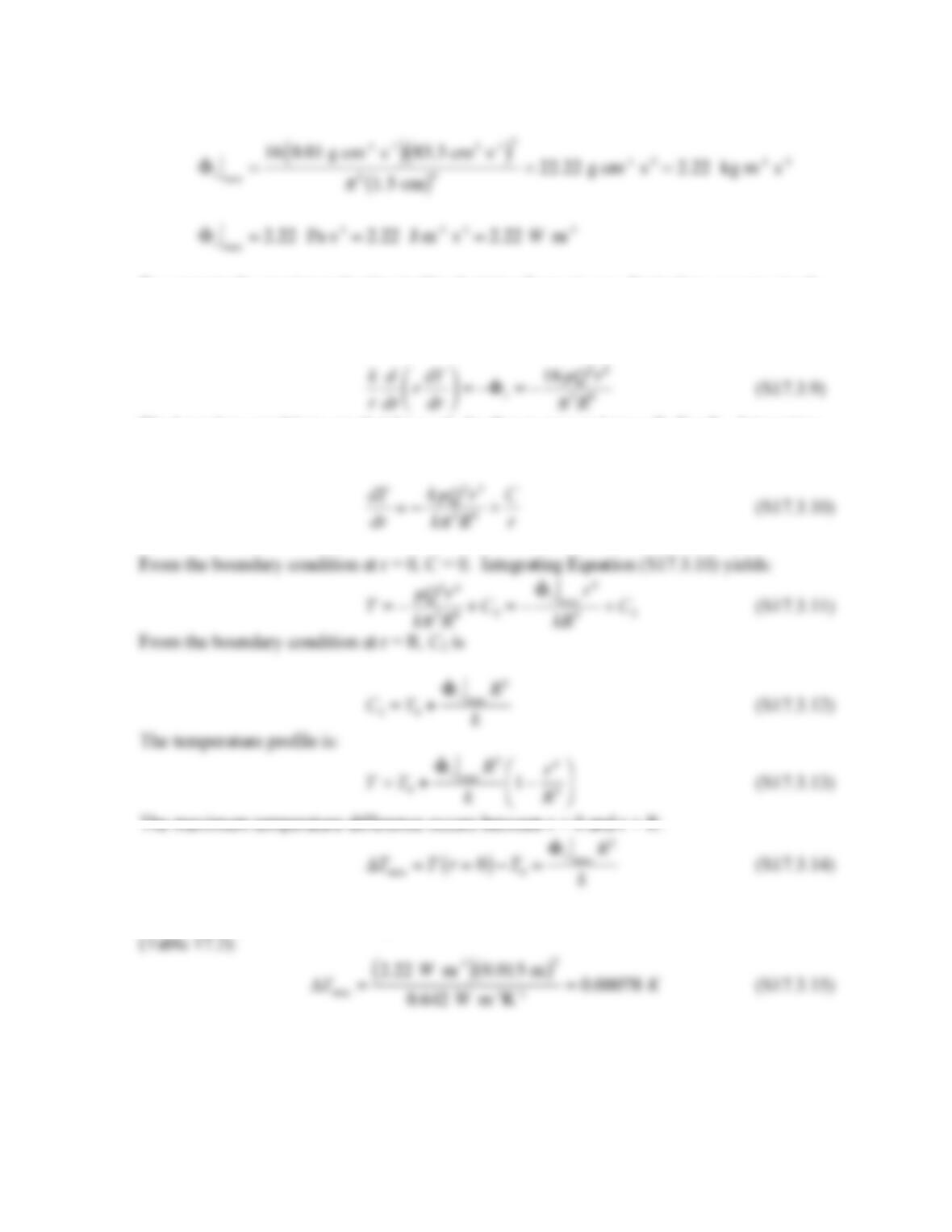
For the value of the viscous dissipation obtained above and the thermal conductivity of blood
(Table 17.2):
2
Thus, viscous dissipation has a very minor effect on the temperature of blood and can be
neglected.
231
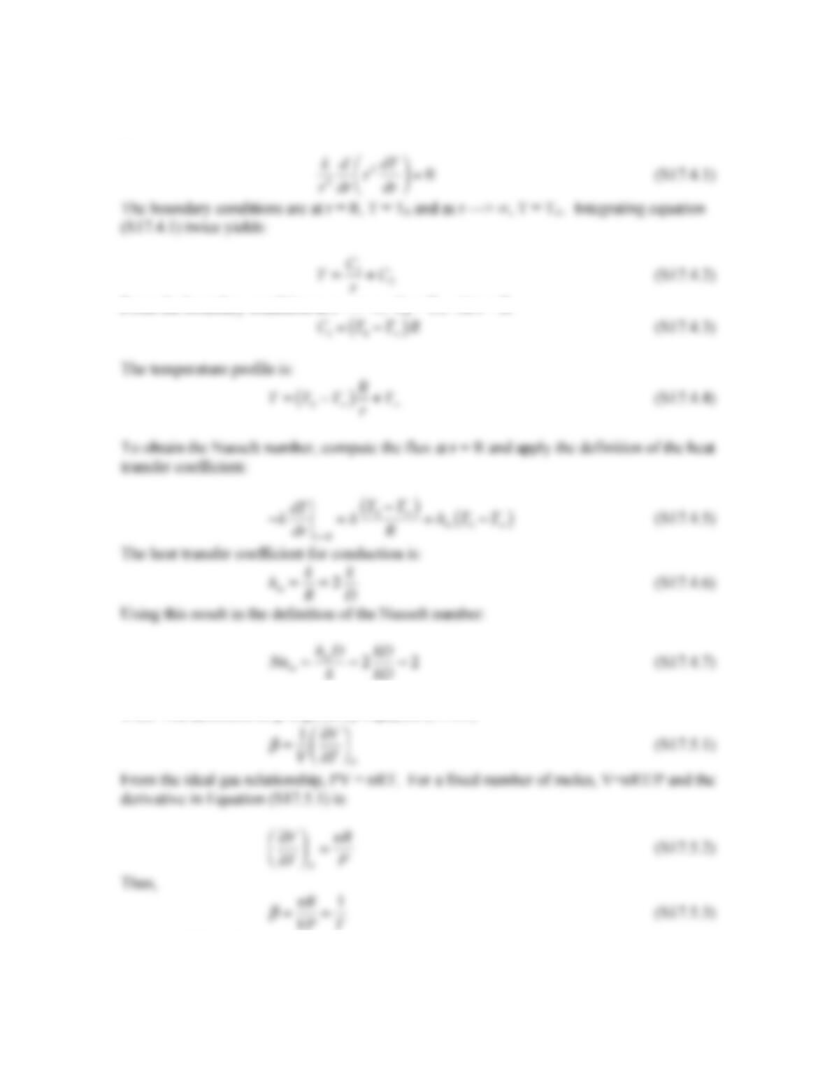
17.4. For steady conduction for a spherical surface of radius R, Equation (17.2.14c) simplifies
to:
k
d
!
From the boundary condition as r —> ∞, C2 = T∞. At r = R
C1=T0!T“
( )
R
(S17.4.3)
17.5. The definition of β is given by Equation (17.4.7)
!
=1
V
“V
“T
#
$
%&
‘
(
P
(S17.5.1)
since T = PV/nR for an ideal gas.
232
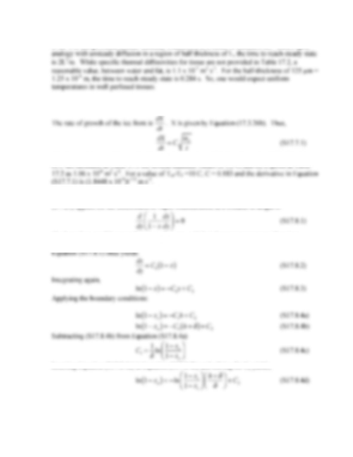
17.6. For this problem, assume unsteady conduction in a tissue of thickness 2L. Based upon
analogy with unsteady diffusion in a region of half thickness of L, the time to reach steady state
is 2L2/α. While specific thermal diffusivities for tissue are not provided in Table 17.2, a
17.7. Note: The phase change during freezing is discussed in Section 17.3.4, not Section 17.3.3.
The rate of growth of the ice front is
dX
dt
. X is given by Equation (17.3.26b). Thus,
C is dimensionless and is provided by solving Equation (17.3.31) or Equation (17.3.33). Values
of C are tabulated in Table 17.3 for several different values of Tm-T0 and αS is given in Table
17.2 as 1.06 x 10⁻⁶ m2 s-1. For a value of Tm-T0 =10 C, C = 0.183 and the derivative in Equation
(S17.7.1) is (1.8448 x 10⁻⁴)t-1/2 m s-1.
17.8. This problem is a modification of the problem presented in Example 6.6. Thus, Equation
(6.7.25) applies for the distribution of vapor concentration in a column of height δ.
d
dy
1
1!x
dx
dy
“
#
$%
&
‘=0
(S17.8.1)
The boundary conditions are that, at y = h, x = xa which is the vapor pressure at the given
temperature and pressure. At y = h + δ, x = xs, the relative humidity in the air. Integrating
Equation (S17.8.1) once yields:
dx
Inserting Equation (S17.8.4c) in Equation (S17.8.4b) and solving for C2 yields;
ln 1 !xa
( )
=!ln 1!xs
1!xs
“
#
$%
&
‘
h+
(
(
“
#
$%
&
‘+C2
(S17.8.4d)
233
C2=ln 1 !xa
( )
+ln 1!xs
1!xa
“
#
$%
&
‘
h+
(
(
“
#
$%
&
‘
(S17.8.4d)
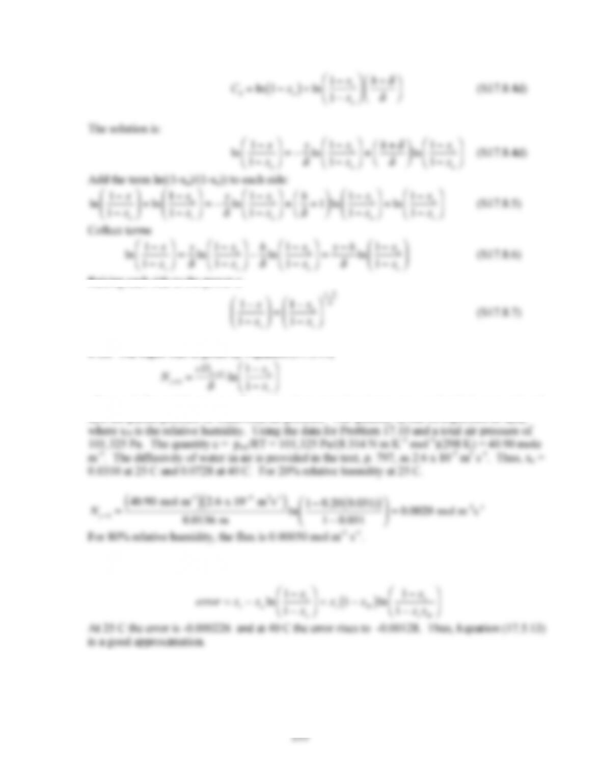
The solution is:
ln 1!x
1!xa
“
#
$%
&
‘=!y
(
ln 1!xs
1!xa
“
#
$%
&
‘+h+
(
(
“
#
$%
&
‘ln 1!xs
1!xa
“
#
$%
&
‘
(S17.8.4d)
Add the term ln((1-xa)/(1-xs)) to each side:
ln 1!x
1!xa
“
#
$%
&
‘+ln 1!xa
1!xs
“
#
$%
&
‘=!y
(
ln 1!xs
1!xa
“
#
$%
&
‘+h
(
+1
“
#
$%
&
‘ln 1!xs
1!xa
“
#
$%
&
‘+ln 1!xa
1!xs
“
#
$%
&
‘
(S17.8.5)
Collect terms
ln 1!x
1!xs
“
#
$%
&
‘=y
(
ln 1!xa
1!xs
“
#
$%
&
‘!h
(
ln 1!xa
1!xs
“
#
$%
&
‘=y!h
(
ln 1!xa
1!xs
“
#
$%
&
‘
(S17.8.6)
Raising each side to the power e:
1!x
1!xs
“
#
$%
&
‘=1!xa
1!xs
“
#
$%
&
‘
y!h
(
(S17.8.7)
17.9. The vapor flux is given by Equation (17.5.11)
Ny=h=cDw,air
!
ln 1“xa
1“xs
#
$
%&
‘
(
where xs is the partial pressure of water in air at saturation (vapor pressure/total air pressure) and
xa is the partial pressure of water/total air pressure. The quantity xa can be expressed as xHxs,
where xH is the relative humidity. Using the data for Problem 17.10 and a total air pressure of
101,325 Pa. The quantity c = ptot/RT = 101,325 Pa/(8.314 N m K-1 mol-1)(298 K) = 40.90 mole
17.10. The error can be computed from the ratio of Equations (17.5.12) to Equation (17.5.13):
17.11. Since the enthalpy of vaporization is a function of temperature, application of Equation
(17.5.25) or Equation (17.5.26) is done iteratively. That is, the enthalpy of vaporization is
updated, once the temperature at the air-sweat interface is calculated. The flux for the
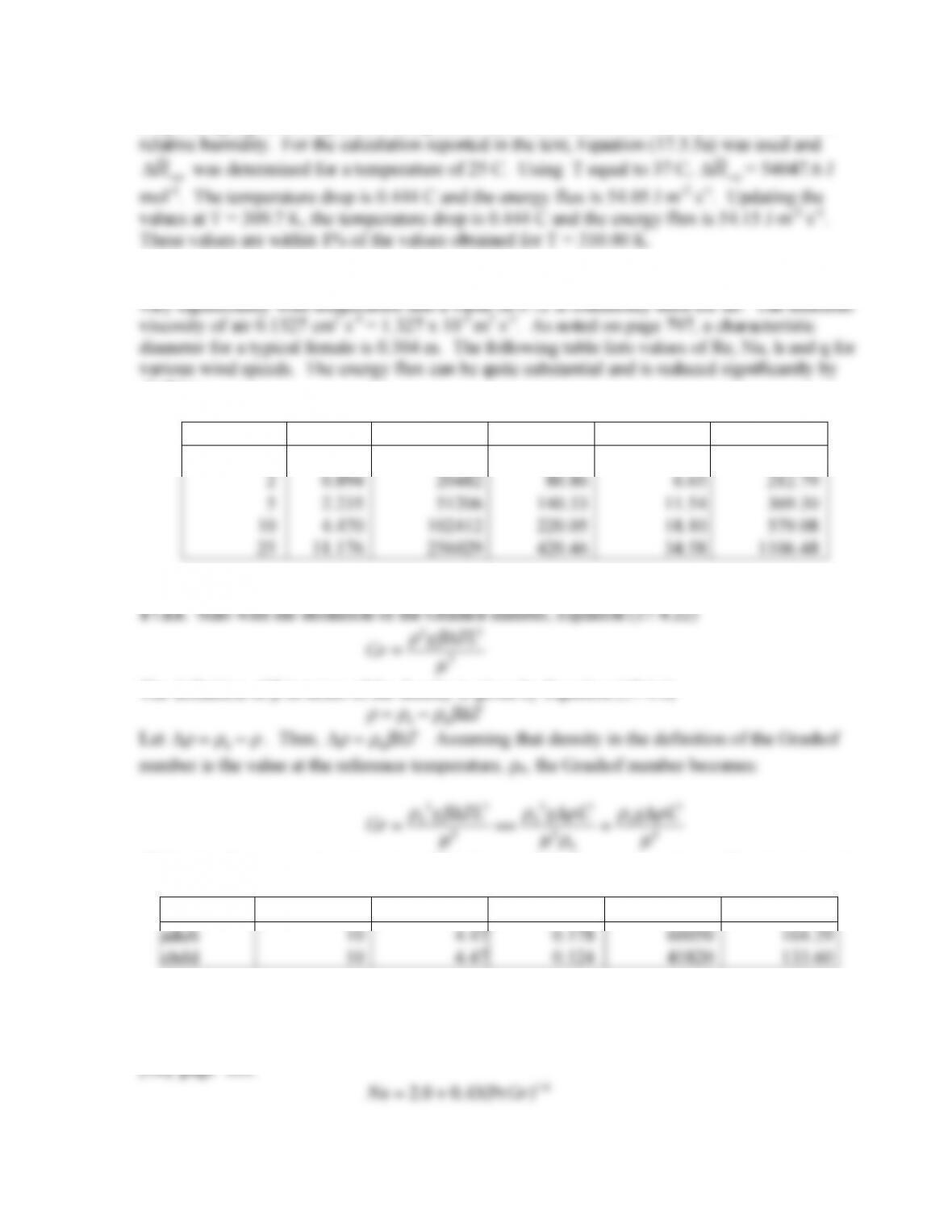
234
evaporating liquid is temperature independent and was found to be 0.001 mol m-2 s-1 for 60%
relative humidity. For the calculation reported in the text, Equation (17.5.5a) was used and
!Hvap
was determined for a temperature of 25 C. Using T equal to 37 C,
!Hvap
= 54047.6 J
17.12. Use Equation (17.4.3) to calculate the Nusselt number. The Prandtl number does not
vary significantly with temperature and a value of 0.72 is commonly used for air. The kinemtic
viscosity of air 0.1327 cm2 s-1 = 1.327 x 10⁻⁵ m2 s-1. As noted on page 797, a characteristic
v, miles/h
v, m/s
Re
Nu
h, W m-2 K-1
q, W m-2
1
0.447
10241
54.64
4.49
143.80
2
0.894
20482
80.86
6.65
212.79
5
2.235
51206
140.33
11.54
369.30
17.13. Start with the definition of the Grashof number, Equation (17.4.22)
!
2g
“
#TL3
The definition of β in terms of the density is given by Equation (17.4.6)
!
“
!
0#
!
0
$
%T
Let
!
“
=
“
0#
“
. Thus,
!
“
#
“
0
$
!T
. Assuming that density in the definition of the Grashof
number is the value at the reference temperature, ρ0, the Grashof number becomes:
Gr =
!
0
2g
“
#TL3
µ
2==
!
0
2g#
!
L3
µ
2
!
0
=
!
0g#
!
L3
µ
2
17.14. For free convection, Equation (17.4.5) is used for flow over a sphere. The viscosity ratio
is 0.900 and Pr = 0.72.
v, miles/h
v, m/s
Diameter, m
Re
Nu
adult
10
4.47
0.178
60050
164.29
child
10
4.47
0.124
41820
133.60
For free convection, the Grashof number is calculated using Equation (17.4.22) with L equal to
the diameter and β = 1/T where T is the air temperature (273.15 K). Equation (17.4.24) is used
to determine the Nusselt number for a flat plate. The correlation for spheres is found in reference
[18], page 301.
Nu =2.0 +0.43(Pr Gr)1/ 4
235
Diameter, m
Gr
Nu, flat plate
Nu, sphere
adult
0.178
42697290
38.57
34.02
child
0.124
14422151
29.40
26.41
For radiation, the energy flux is given by Equation (17.2.19c). Treating the absorptivity and
emissivity as the same, the flux equals q = σe(Tb4–Tair4). A heat transfer coefficient can be
defined as h=q/ΔT and a Nussel number determined. Results are:
qrad
h
Nu adult
Nu child
193.44
5.23
37.22
25.93
Comparing results, the free convection and radiation terms are comparable and are about 20% of
the value for forced convection.
17.15. Note, there is a typographical error in the text and Equation (17.5.25) should be:
ˆ
ˆ
kl
Cvapka
$
%&
‘
( “1“exp
Cvap ka
$
%&
‘
(
,
–
/
0
Begin with Equation (17.5.21) for air and Equation (17.5.24) for the liquid.
T
a=a1Cvapka
Ny=h
!
ˆ
Cp
exp
!
ˆ
Cp
Cvap ka
Ny=hy
“
#
$%
&
‘+a2
(17.5.21)
The boundary conditions are:
y = 0 Tl = Tb (S17.15.1a)
y = h Tl = Ta (S17.15.1b)
From the boundary condition at y = 0
a4=T
b
(S17.15.2a)
236
a2=T
air !a1Cvapka
Ny=h
“
ˆ
Cp
exp
“
ˆ
Cp
Cvap ka
Ny=hh+
#
( )
$
%
&‘
(
)
(S17.15.3a)
Use Equations (S17.15.3b) and (S17.15.5) to compute the derivatives of the temperature. The
boundary condition, Equation (S17.15.1c), becomes:
ˆ
“
)kla1Cvapka
hNy=h
!
ˆ
Cp
exp
Cvap ka
Ny=hh
#
$%
&
‘1)exp
Cvap ka
Ny=h
*
#
$%
&
‘
,
–
–
/
0
0
=(Hvap Ny=h
Solving for a1:
a1=
exp !
“
ˆ
Cp
Cvap ka
Ny=hh
#
$
%&
‘
()Hvap Ny=h!kl)T
h
#
$
%&
‘
(
ka !klCvapka
hNy=h
“
ˆ
Cp
1!exp
“
ˆ
Cp
Cvap ka
Ny=h
*
#
$
%&
‘
(
+
,
–
–
.
/
0
0
(S17.15.7)
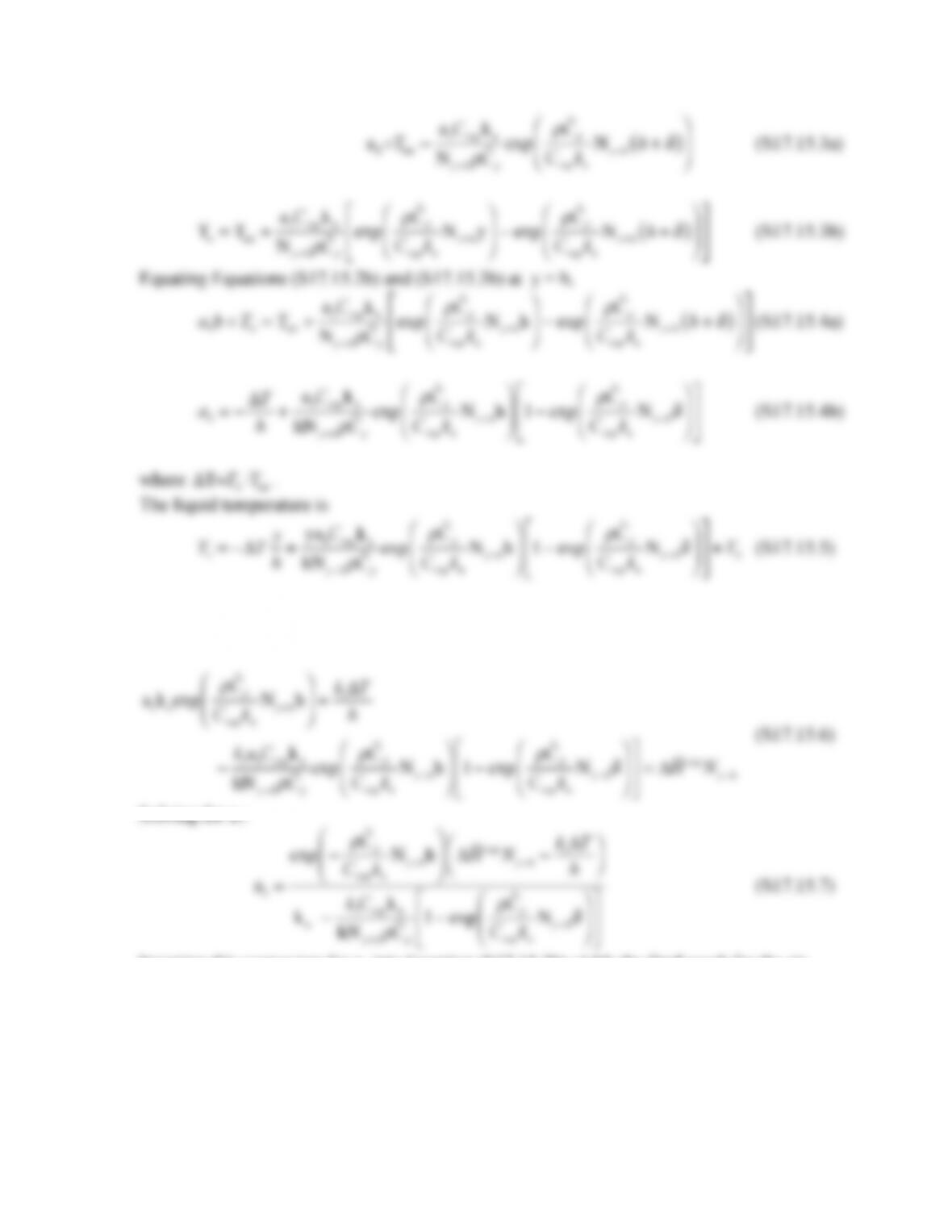
Inserting this expression for a1 into Equation (S17.15.3b) yields the final result for the air
temperature.
237
T
a=T
air +!Hvap Ny=h“kl!T
h
#
$
%&
‘
(
Cvapka
Ny=h
)
ˆ
Cp
exp
)
ˆ
Cp
Cvap ka
Ny=hy-h
( )
#
$
%&
‘
(“exp
)
ˆ
Cp
Cvap ka
Ny=h
*
#
$
%&
‘
(
+
,
–
–
.
/
0
0
ka “klCvapka
hNy=h
)
ˆ
Cp
1“exp
)
ˆ
Cp
Cvap ka
Ny=h
*
#
$
%&
‘
(
+
,
–
–
.
/
0
0
(S17.15.8a)
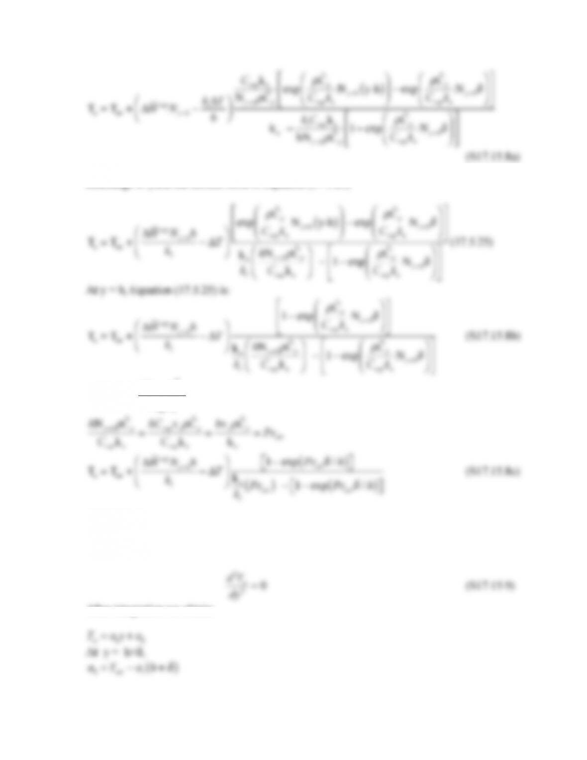
Rearrange to yield the correct form of Equation (17.5.25)
ˆ
ˆ
kl
Cvapka
$
%&
‘
( “1“exp
Cvap ka
$
%&
‘
(
,
–
/
0
The group
hNy=h
!
ˆ
Cp
Cvapka
can be rewritten as the following by using Equation (17.5.17):
hNy=h
!
ˆ
Cp
Cvapka
=hCvapvy
!
ˆ
Cp
Cvapka
=hvy
!
ˆ
Cp
ka
=Peair
T
a=T
air +!Hvap Ny=hh
kl
” !T
#
$
%&
‘
(1“exp Peair
)
/h
( )
*
+,
–
ka
kl
Peair
( )
“1“exp Peair
)
/h
( )
*
+,
–
(S17.15.8c)
The thermal Peclet number for air is 0.20, which is larger than the value for sweat, but still much
less than 1. For the case of conduction only, energy transport through the liquid is unchanged.
Equation (17.5.17) for the air simplifies to:
d2Ta
After integration we obtain:
Ta=a1y+a2
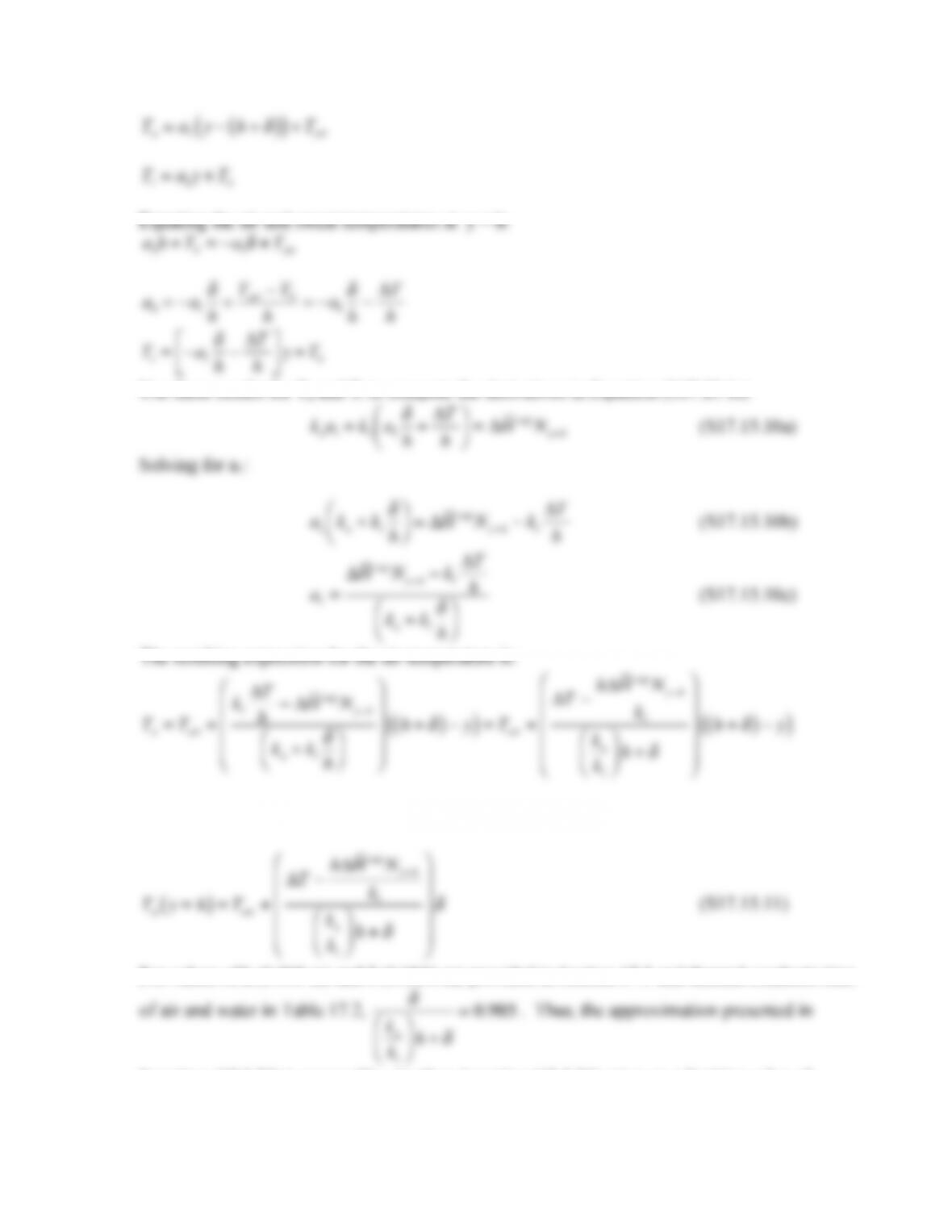
238
Ta=a1y!h+
“
( )
( )
+Tair
Tl=a3y+Tb
Equating the air and sweat temperatures at y = h:
a3h+Tb=!a1
“
+Tair
a3=!a1
“
h
+Tair !Tb
h
=!a1
“
h
!#T
h
Tl=!a1
“
h
!#T
h
$
%
&‘
(
)y+Tb
Use these results for Ta and Tl to compute the derivatives in Equation (S17.15.1c)
kaa1+kla1
!
h
+“T
h
#
$
%&
‘
(=“Hvap Ny=h
(S17.15.10a)
h
%
(
%
(
kl
%
&‘
(
)h+
%
(
for y = h
kl
$
%&
‘
(h+
$
‘
For values of h (0.005 m) and δ (0.0136 m) provided in Section 17.5 and thermal conductivities
of air and water in Table 17.2,
!
ka
kl
“
#
$%
&
‘h+
=0.985
. Thus, the approximation presented in
Equation (17.5.26) is reasonable. Further, Equation (17.5.26) arises as a limiting value of
Equation (17.5.25) when ka/klPe << 1.
239
If vaporization does not occur, then
!Hvap =0
and Equation (17.5.27) results.
17.16. From Table 2.4, the blood vessel diameters range from 6 x 10⁻⁶ m to 5 x 10⁻⁵ m.
Corresponding mean velocities range from 2 x 10⁻⁴ to 0.001 m s-1. The Pe ranges from 0.0068 to
0.284. Blood vessel densities range from 2.0 x 10⁸ vessels m-2 to 2.22 x 10⁹ vessels m-2. The