
SOLUTIONS TO CHAPTER 16 PROBLEMS
Decision Tree Analysis
16-1.
195
16-2.
196
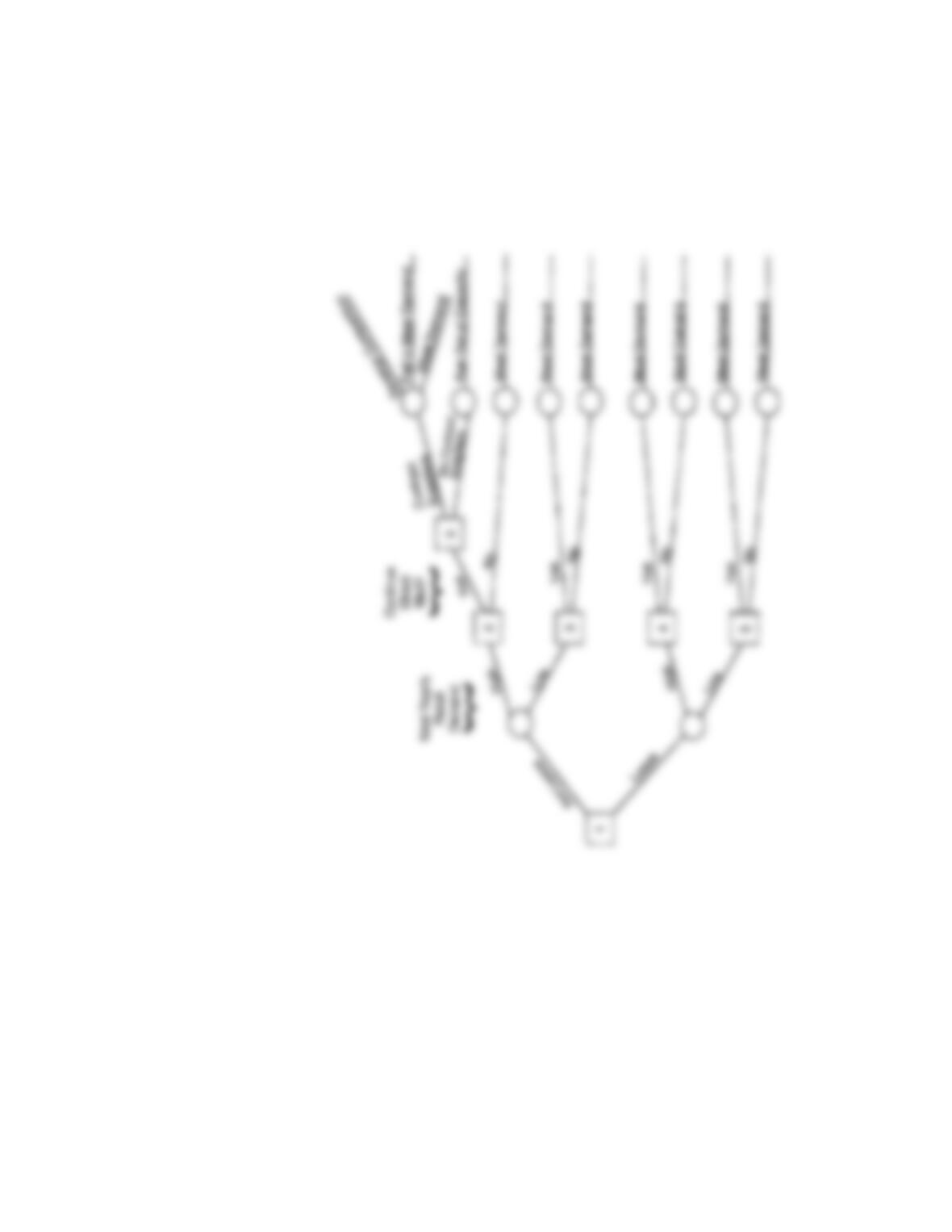
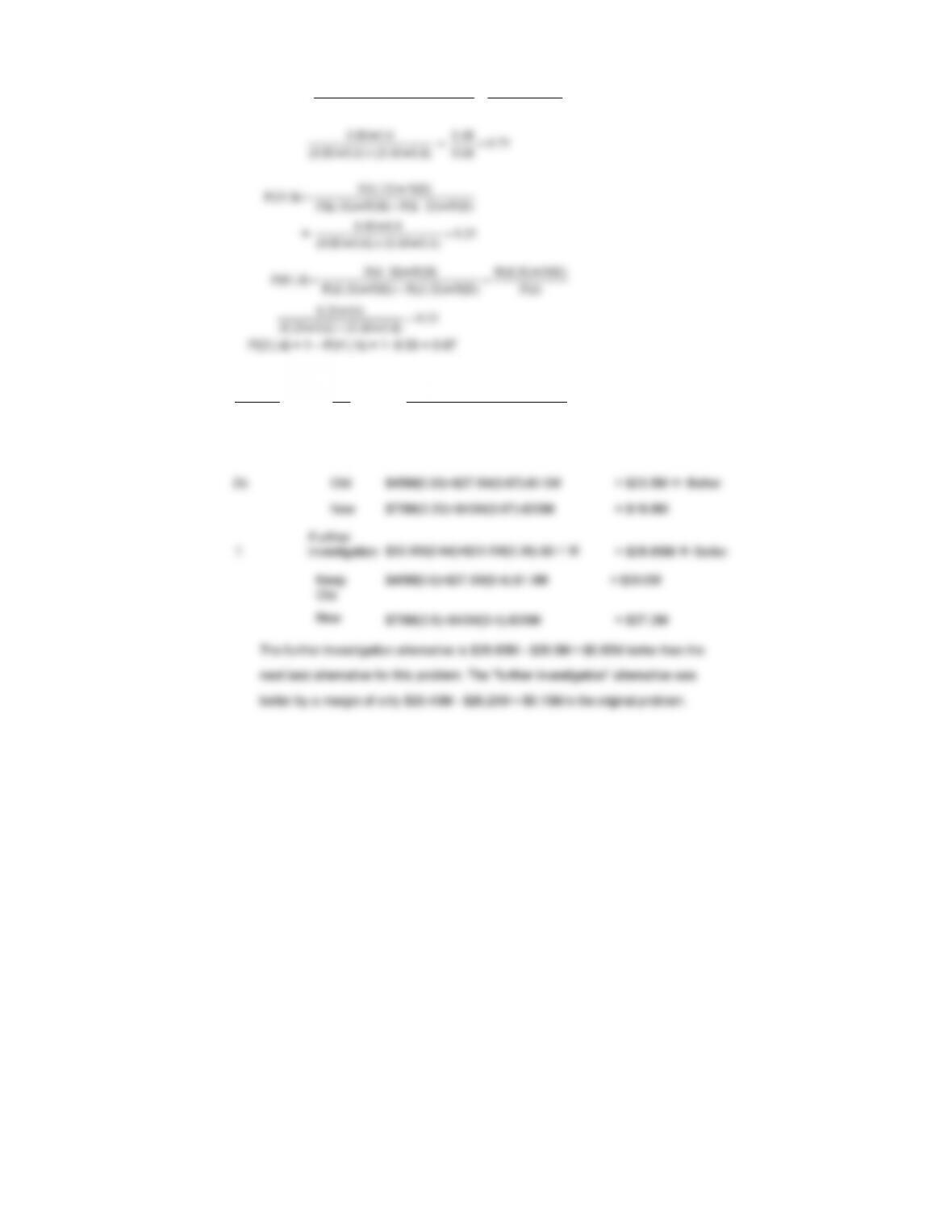
16-3. (a) M – thousands
197
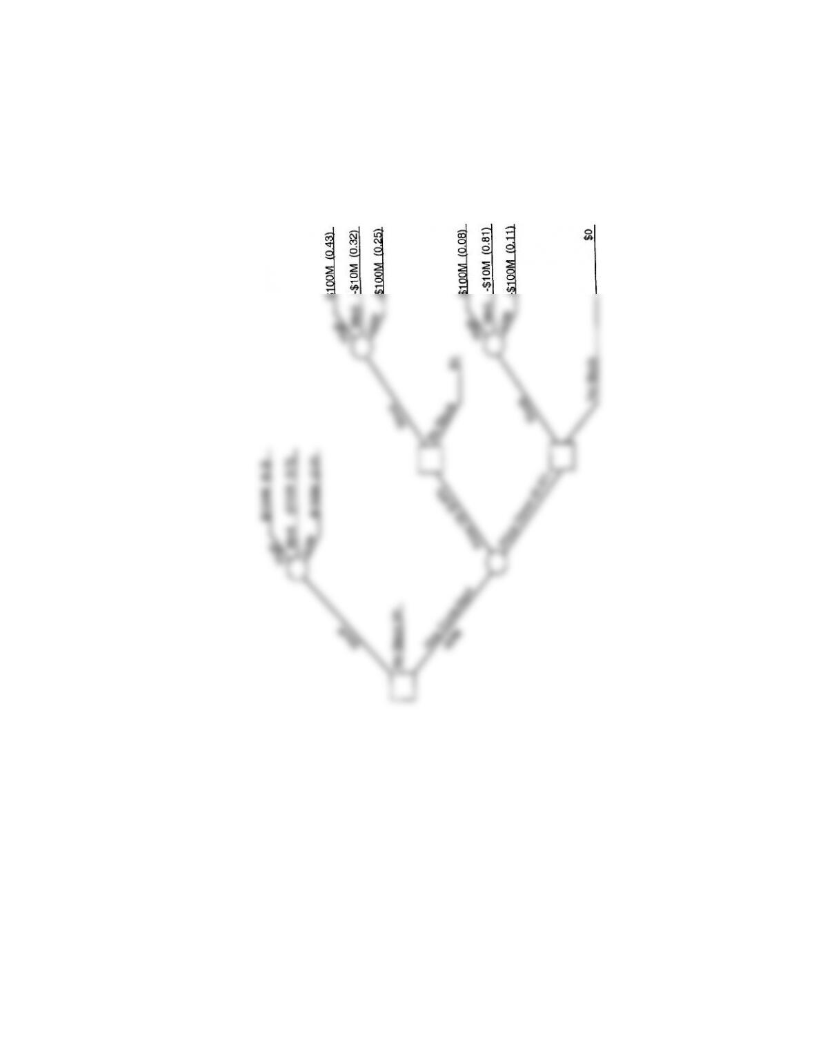
16-3. (continued)
(b) Posterior Probabilities, Given Prediction Price Will Go Up, (u)
(1) (2) (3) (4)=(2)(3)
(5)=(4)/ ∑(4)
(Price) P(Price) P(u l Price) Joint Probab. P (Price l u)
High 0.3 0.9 0.27 0.43
Dec. 2:
Stock: $100M(0.43) – $10M(0.32) – $100M(0.25) = $14,800 Å Better
No Stock: = $0
198
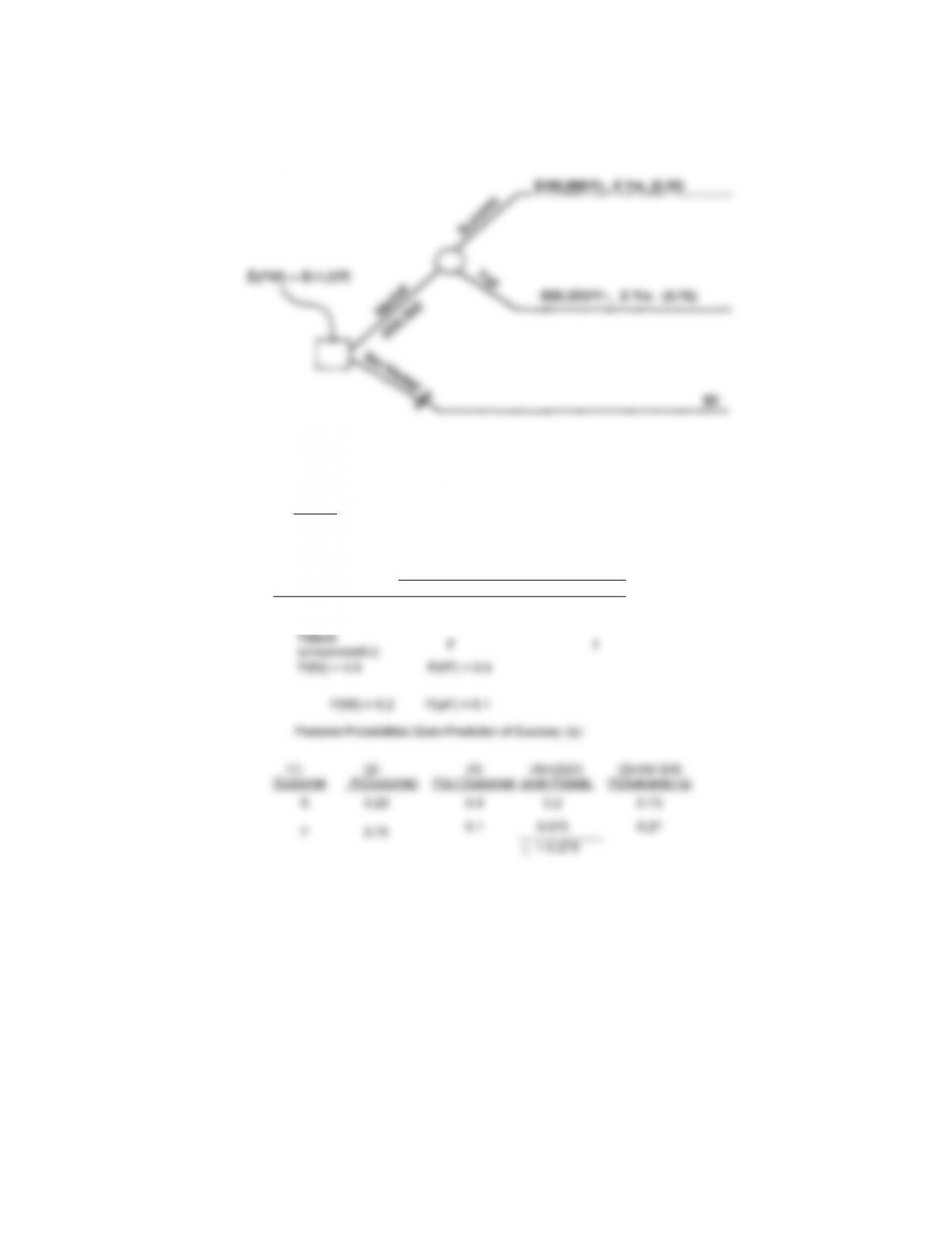
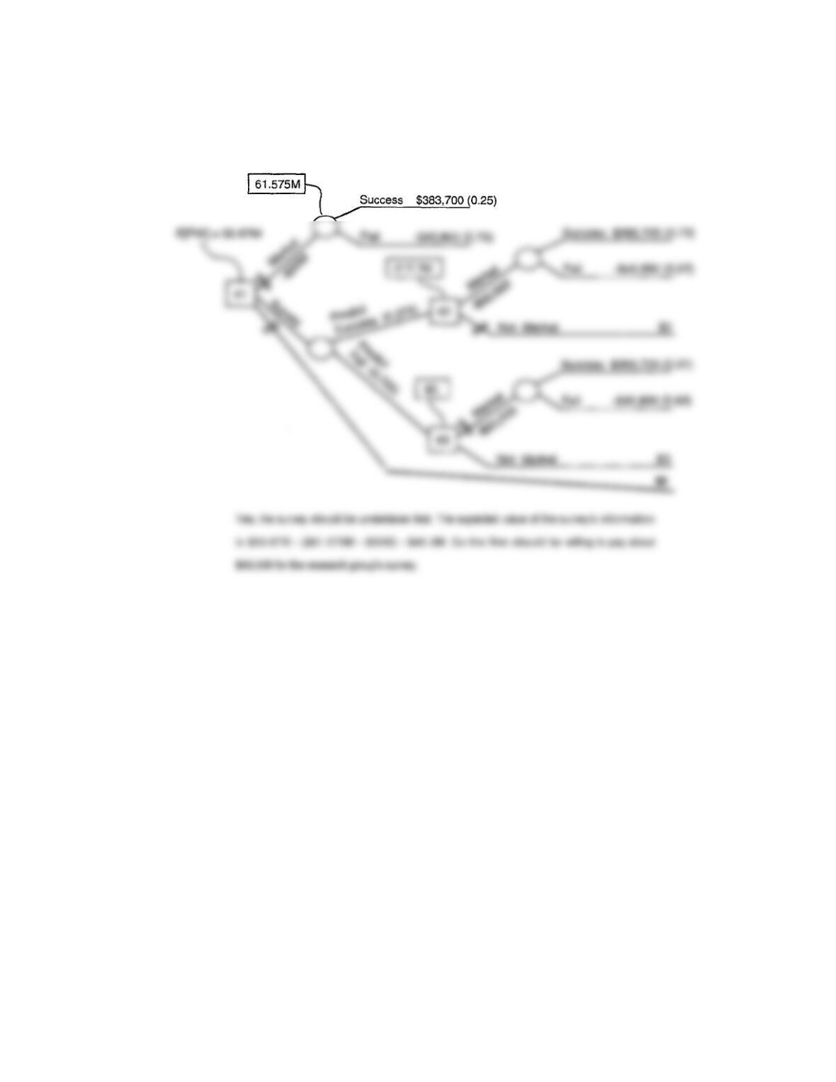
16-4. (a)
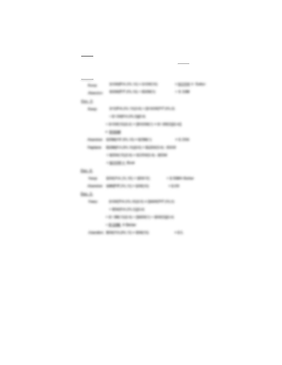
PW(Success) = $100,000(P/A,20%,8) = $383,700
PW(Fail) = -$30,000(P/A,20%,2) = -$45,800
Market:
E(PW) = $383,700(0.25) – $45,800(0.75) – $50,000 = $11,575
(b) Outcome SYMBOL
Actual Outcome Prediction
Successful S s
199
16-4. (continued)
Posterior Probabilities, Given Prediction of Failure, (f):
Outcome P(Outcome) P(f l Outcome) Joint Probab. P(Outcome l f)
S 0.25 0.2 0.05
F 0.75 0.9 0.675
∑ = 0.725
0.07
0.93
200
16-4 (continued)
M — thousands
201
16-5. M ≡ thousands
202
16-5. (continued)
203
16-6. First, analyzing the alternatives at Decision Point 2:
For Alternative NC the present worth of costs is
$1,000(P/A,12%,7)(0.2) + $18,000(P/A,12%,7)(0.8)
204
16-6. (continued)
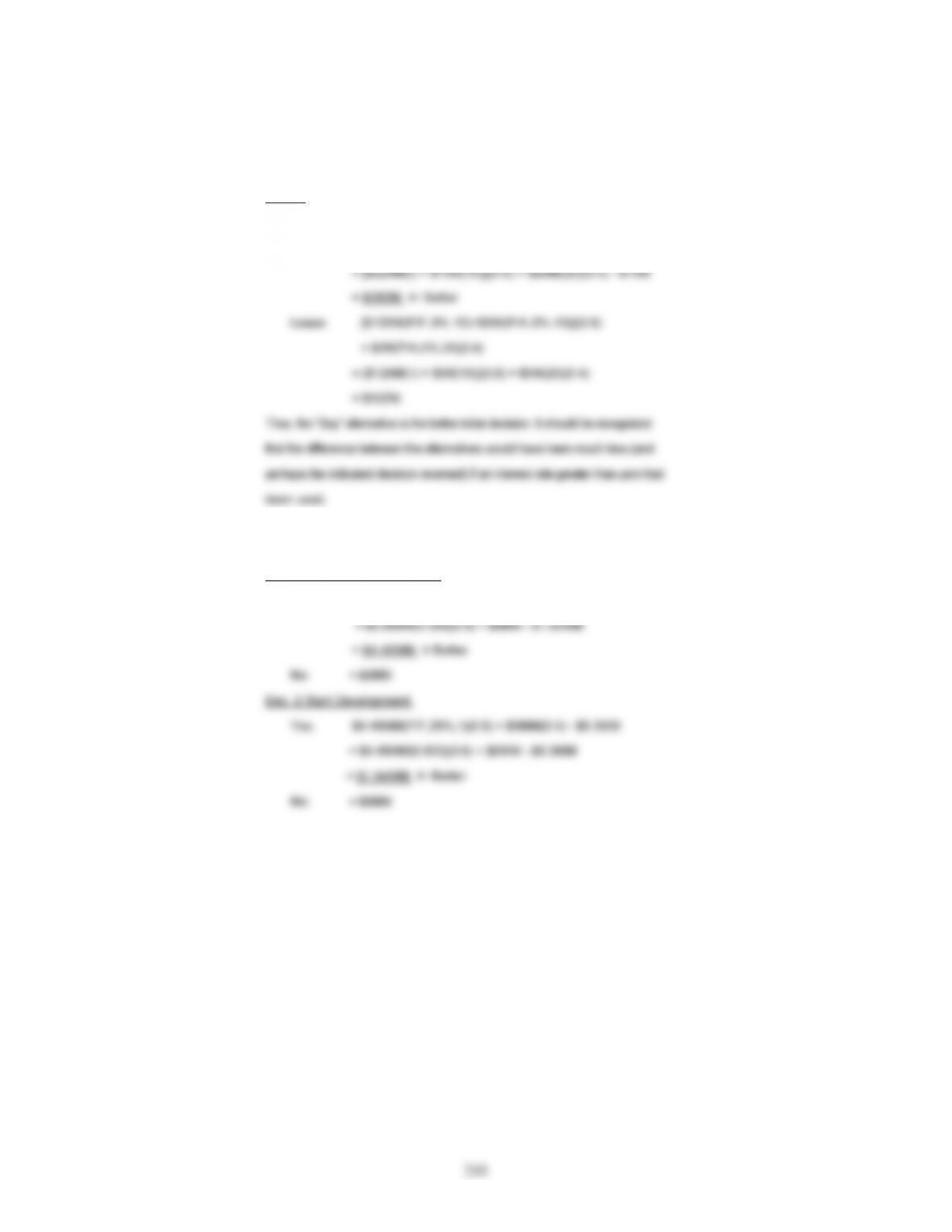
For alternative RLW the present worth of costs is
= $18,000(P/A,12%,10)(0.15) + [$18,000(P/A,12%,3)
205
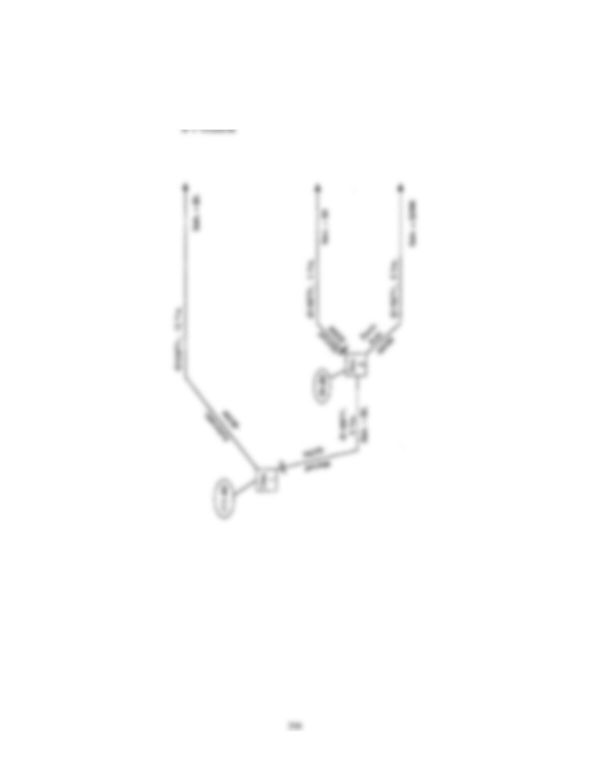
16-7. (a) Decision tree diagram showing outlays (costs) as negative numbers.
(continued)
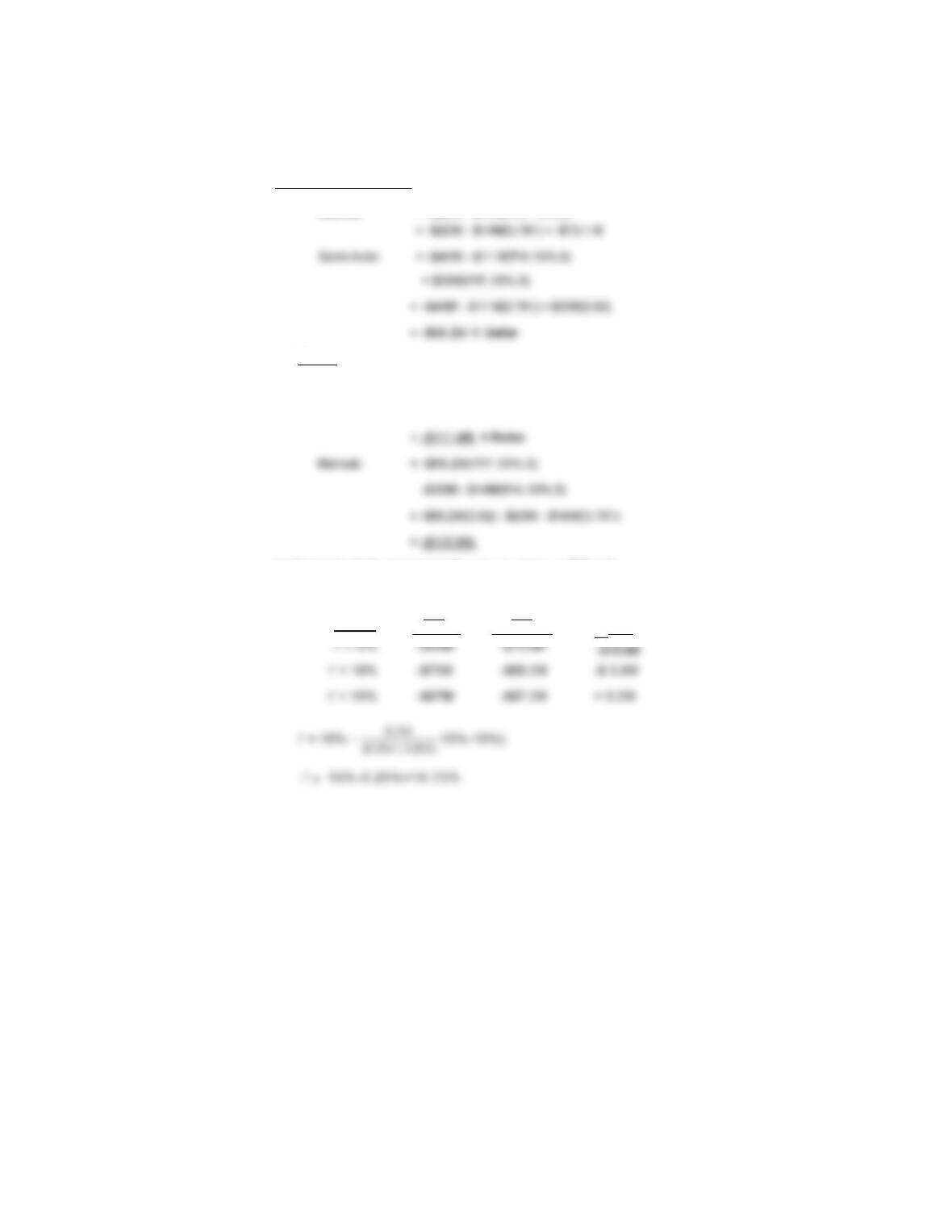
(b) Dec. 2:
16-7.
Manual: = -$20M – $14M(P/A, 10%,5)
Dec. 1:
Automatic: = -$50M – $10M(P/A,10%,10)
= –$50M – $1 0M(6.114)
(c) Find i’ at which present worths are equal (or ∆ PW = 0)
-$20M – $14M(P/A,i’%,5) = -$40M – $11 M(P/A, i’ %,5) + $20M(P/F, i %,5)
Interest PW
(Manual)
PW
(Semi-Auto) ∆ PW
207
16-8. P(h)
P(H) H)|P(h
P(D)D)|P(h P(H)H)|P(h
P(H) H)|P(h
h)|P(H •
=
•+•
•
=
0.48
0.60.80 ==
•
M ≡ thousands
Dec. Pt. Alt. Expected Monetary Outcome
2a Old $45M(0.75)+$27.5M(0.25)-$1 0M = $30.62M
New $75M(0.75)+$43M(0.25)-$35M = $32.0M Å Better
208
$10M(P/A,0%,10) = $1 0M(10) = $100M Å Better
$20M(P/F,0%,10) = $20M(1) = $ 20M
16-9. Note: M ≡ thousands
Dec. 4:
Keep:
Abandon:
Dec. 5:
209
16-9. (continued)
Dec. 1:
Buy: [$220M(P/F,0%,10)+$10M(P/A,0%,10)](0.6)
+ $20M(P/A,0%,25)(0.4) – $100M
16-10. Note: MM = millions
Dec. 3 Start Commercialization:
Yes: $2.00MM(P/A,20%,6)(0.9) + $0MM(0.1) – $1.50MM
16-10. (continued)
Dec. 1 Start Applied Research:
Yes: $1.94MM(P/F,20%,1)(0.5) + $0MM(0.5) – $0.10MM
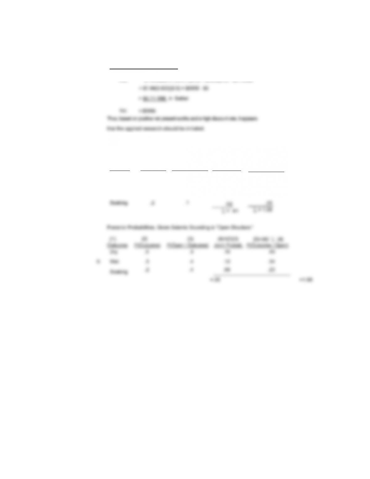
16-11. Posterior Probabilities, Given Seismic Sounding is “No Structure:”
(4)=(2)(3)
Joint Probab.
(3)
P(No l Outcome)
(1)
Outcome
(2)
P(Outcome)
(5)=(4)/ ∑ (4)
P(Outcome l No)
N: Dry
Wet
.5
.3
.6
.3
.30
.09
.73
.22
211
SOLUTIONS TO CHAPTER 17 PROBLEMS
Capital Investment Decisions as Options
17-1. (a) The NPV of 1 million is positive but not over whelmingly so given the size of the proposed investment. Very minor
changes in the estimated costs could make this NPV negative.
17-2. The risk free rate impacts the value of NPVq .
17-3. S =41
X = 60
PV(X) =
t
)2.01/(60 +
17-4. t=1
σ
= 0.4 according to Luehrman
X = 500
S = PV of $150 per year over 19 years
rf = 0.02
212
Option value (0.37)(808)
≈298.96, using 37% as the table value.
0.37 estimated from table 17.1
808 Value of S
17-5. $112M = S
$6M $ 106M = X
17-6. See the concluding section of the chapter, How Far Can You Extend The Framework for many comments on assumptions
and limitations.
213