978-0131206687 Chapter 6 Part 2

118

()()()()

8350.09948.09959.09966.08457.0

p

1o

2o

3o

4o

5o

1o

5o ===

Four oblique shocks:

°=δ

6

9972.0

p

4o

5o

=

Normal Shock

p

6o =

()()()()()

9097.09948.09959.09966.09972.09239.0

p

1o

2o

3o

4o

5o

1o

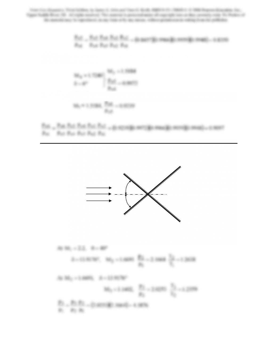
Problem 12. – Two oblique shocks intersect as shown in Figure P6.12. Determine the

flow conditions after the intersection, with γ = 1.4.

Figure P6.12

M = ?

p = ?

T = ?

V = ?

40º

M = 2.2

p = 70 kPa

T = 270 K

this material may be reproduced, in any form or by any means, without permission in writing from the publisher.

119

p

3

⎞

⎛

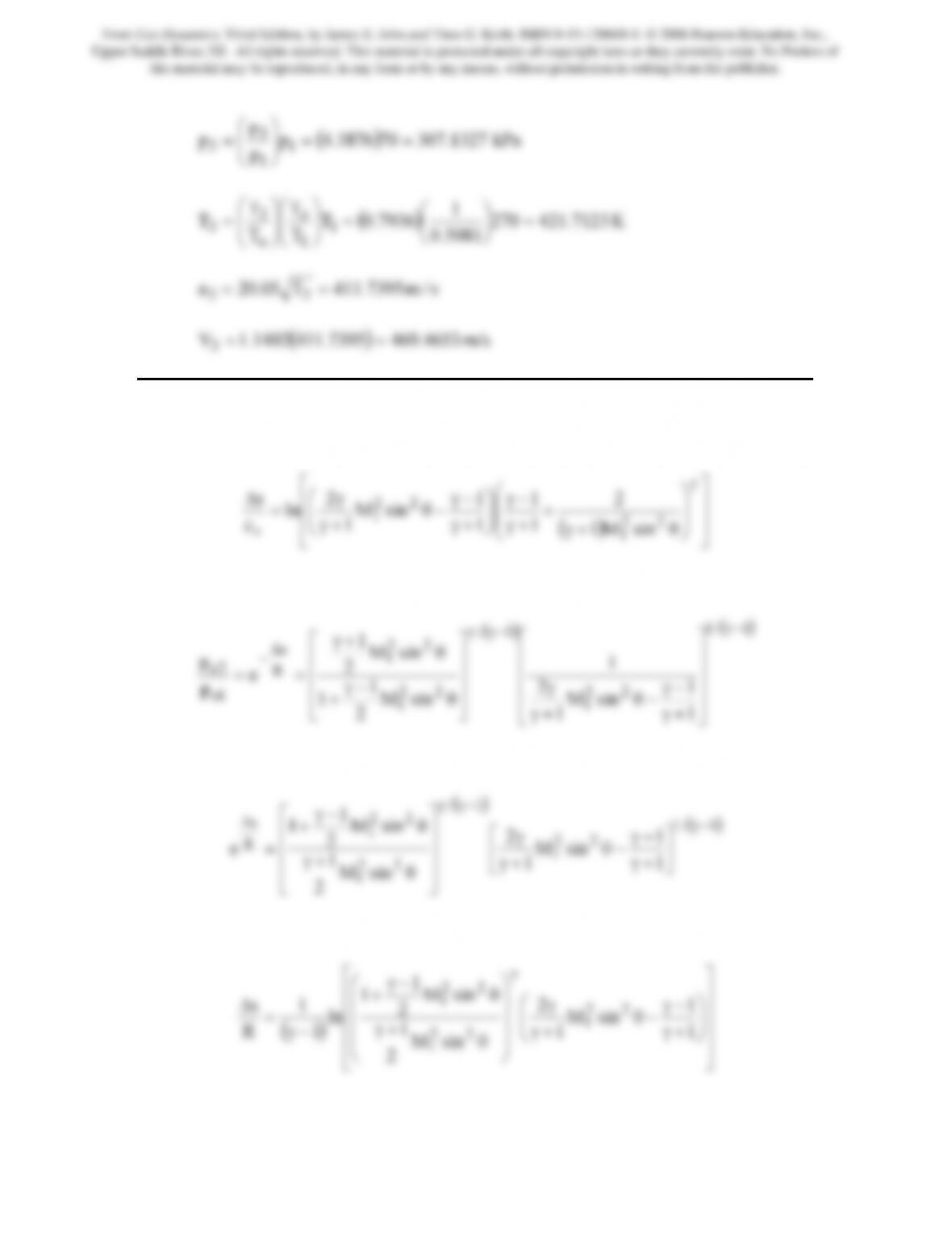
Problem 13. – Show that the entropy increase across an oblique shock is given by,

(Ref. 7)

⎥

⎤

⎢

⎡

⎟

⎞

⎜

⎛

+

−γ

⎟

⎞

⎜

⎛

−γ

−θ

γ

=

∆γ

22

1

2

1

sinM

2

ln

s

From Eq.(6.13)

22

1

22

1

1o

1

sinM

1

2

sinM

2

1

p

⎥

⎦

⎢

⎣

+γ

−γ

−θ

+γ

γ

⎥

⎦

⎢

⎣

θ

−γ

+

and since cv = R/(γ – 1), the above can be written as

1

22

1

sinM

2

1

⎥

⎦

⎢

⎣

+γ

⎥

⎦

⎢

⎣

θ

+γ

So

()

⎥

⎦

⎢

⎣

⎟

⎠

⎜

⎝

+γ

⎟

⎠

⎜

⎝

θ

+γ

−γ

1

sinM

2

1

R

1

22

1

Or

this material may be reproduced, in any form or by any means, without permission in writing from the publisher.

120

⎥

⎤

⎢

⎡

⎟

⎞

⎜

⎛

+

−γ

⎟

⎞

⎜

⎛

−γ

−θ

γ

=

∆γ

22

1

2

1

sinM

2

ln

s

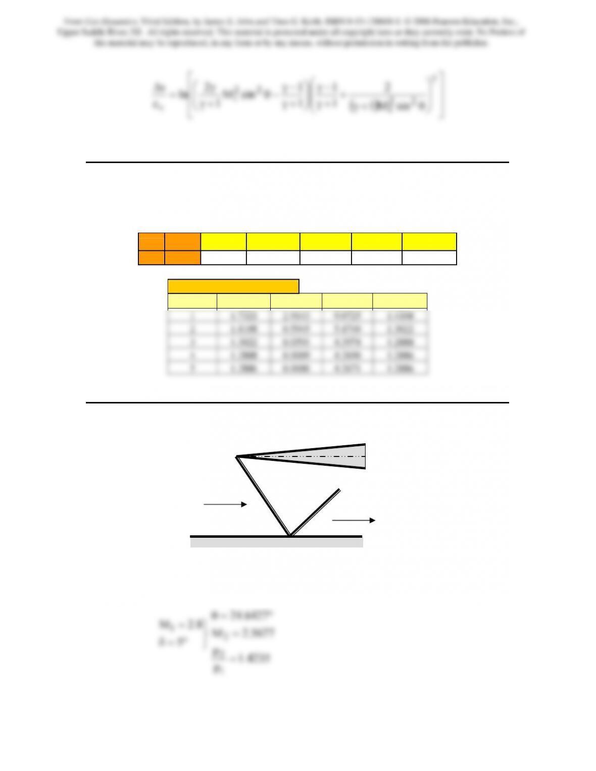
Problem 14. – Repeat the computations of Example 6.2. However, instead of using the

successive substitution method proposed by Collar, and described in Section 6.3, solve

the problem using the Newton-Raphson method.

γ M1 A B C B – AC 1rst guess

1.3 2.0 3.0000 2.9143 0.8870 0.2534 1.7321

Newton-Raphson Method

iteration xold f fprime xnew

Problem 15. – For the two-dimensional case shown in Figure P6.15, determine M3 and

p3. γ = 1.4.

Figure P6.15

⎬

⎫

°=δ

=

5

8.2M1

5677.2M

6427.24

2

=

°=θ

p3 = ?

p1 = 10 kPa

M1 = 2.8

M2 M3 = ?

5º

this material may be reproduced, in any form or by any means, without permission in writing from the publisher.

⎫

=

5677.2M2

7305.26

°

=

θ

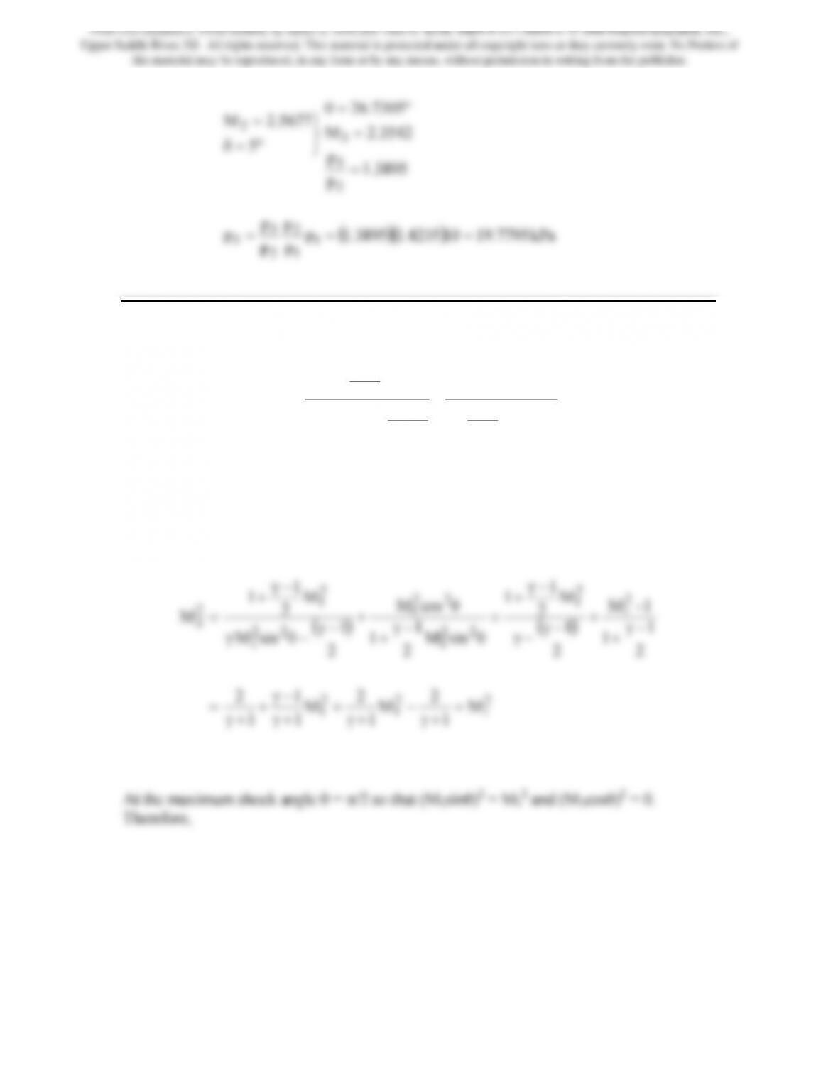
Problem 16. – Prove that: (a) at the minimum shock angle, M2 = M1 and (b) at the

maximum value of the shock angle, Eq.(6.17) becomes Eq.(4.9)

()

θsinM

2

1γ

1

θcosM

2

1γ

θsinMγ

M

2

1γ

1

M

22

1

22

1

22

1

2

1

2

2−

+

−

+

= (6.17)

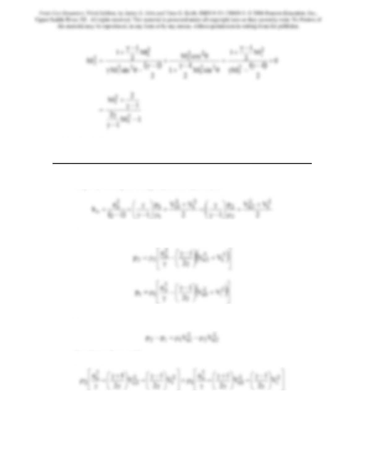
(a) at the minimum shock angle

The minimum shock angle is the angle of a Mach wave for which θ = sin−1(1/M1).

Accordingly, (M1sinθ)2 = 1 and (M1cosθ)2 = M12 – 1. Therefore,

−

2

1

2

1

2

1

M

1

2

M

1

2

M

1

2

=

+γ

−

+γ

+

+γ

−γ

+

+γ

=

(b) at the maximum value of the shock angle

this material may be reproduced, in any form or by any means, without permission in writing from the publisher.

122

0

M

2

1γ

1

θcosM

M

2

1γ

1

M

2

1

22

1

2

1

2

+

−

+

=

+

−

+

=

which is Eq.(4.9).

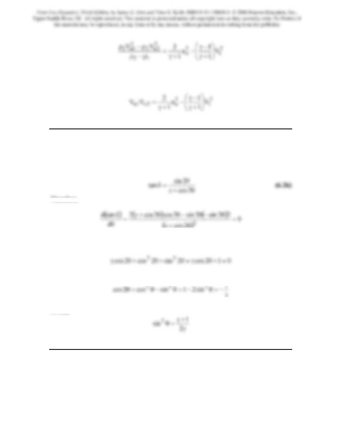
Problem 17. –Develop Prandtl’s relation for oblique shocks from conservation principles.

Begin by writing the energy equation, Eq.(6.5c), as

()

2

12

11

2

1

o

ρ

⎟

⎠

⎜

⎝

−γ

ρ

⎟

⎠

⎜

⎝

−γ

Thus,

⎤

⎡+

⎞

⎛

−γ

22n

2

o

1

a

⎥

⎦

⎢

⎣

⎟

⎠

⎜

⎝

γ

t

1n

11 VV

2

From the momentum equation, Eq.(6.5b),

Combining these yields

⎥

⎦

⎢

⎣

⎟

⎠

⎜

⎝

γ

⎟

⎠

⎜

⎝

γ

⎥

⎦

⎢

⎣

⎟

⎠

⎜

⎝

γ

⎟

⎠

⎜

⎝

γ

2

Rearrangement gives

this material may be reproduced, in any form or by any means, without permission in writing from the publisher.

123

t

o

12

22n2

2

1n1 V

1

a

1

⎟

⎠

⎜

⎝

+γ

−

+γ

=

ρ−ρ

Using the continuity equation, Eq.(6.5a), the expression can be simplified to

obtain Prandtl’s relation for an oblique shock wave

t

o2n1n V

1

⎠

⎜

⎝

+γ

Problem 18. – The largest deflection angle for the limiting upstream Mach number,

M1 → ∞, can be found by differentiating Eq.(6.26), setting the result to zero and then

solving for θ. In other words, verify that Eq.(6.27) is correct.

From Example 6.4 it was shown that

θ

Therefore,

θ

−

θ

−

θ

+

γ

()

2cos

d

θ+γ

θ

Cancel the 2 and rewrite the numerator as

Therefore,

γ

−=θ−=θ−θ=θ 1

sin21sincos2cos 222

So that

γ

+

γ

=θ 2

1

sin2

Problem 19. – In general, the angle of incidence, θi, and the angle of reflection, θr, of an

oblique shock reflected from a flat surface are not equal. However, see Refs. 8 and 9,

there is an angle θ* such that the two angles are equal. Also, if θi < θ*, then (θr – δ) < θi,

and if θi > θ*, then (θr – δ) > θi. Computationally verify that for M1 = 2, 3 and 4 at

γ = 1.4, the angle of incidence and the angle of reflection of an oblique shock reflected

from a flat surface will be equal if

this material may be reproduced, in any form or by any means, without permission in writing from the publisher.

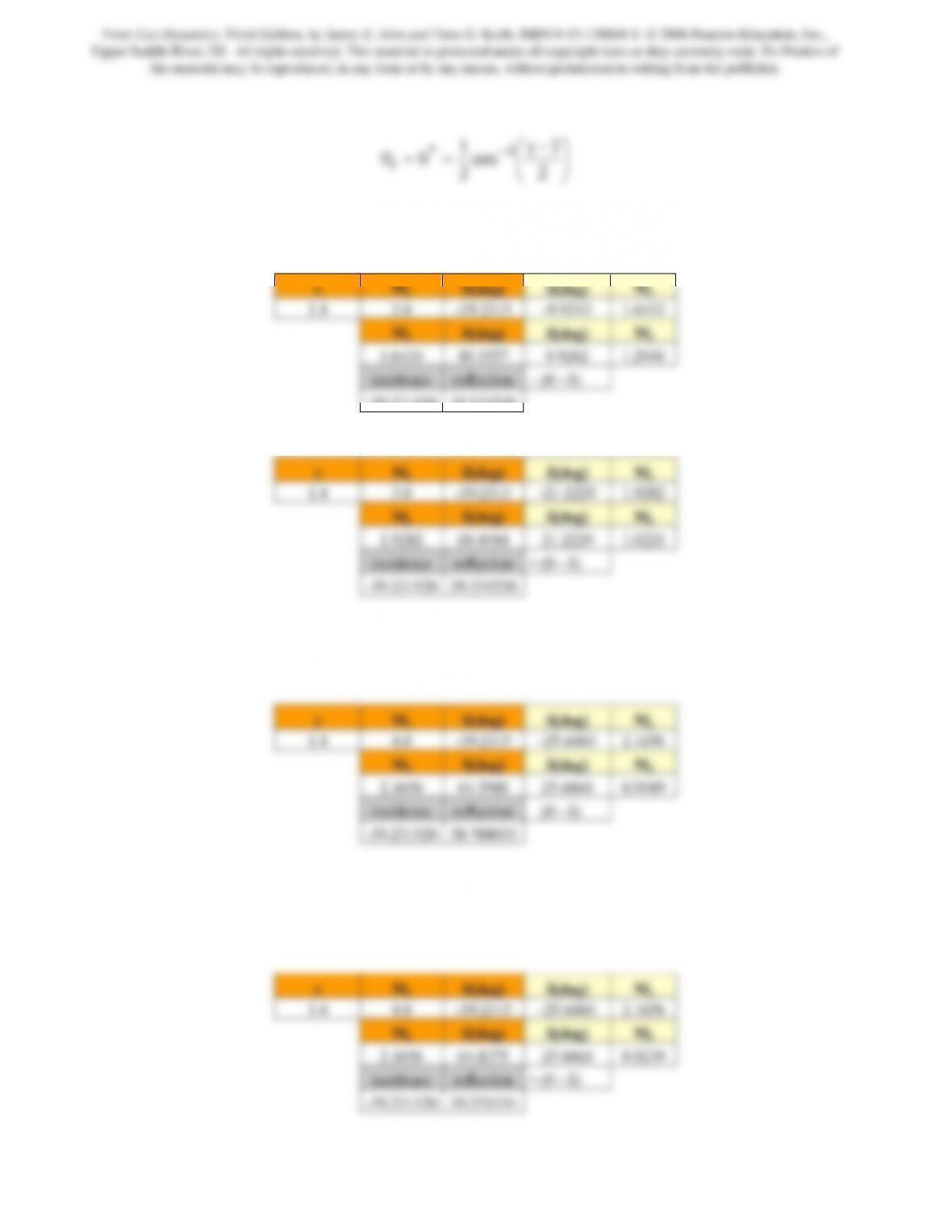
At M1 = 2 and γ = 1.4, the computations yield the following values

-39.231520 39.231520

At M1 = 3 and γ = 1.4, the computations yield the following values

Note the flow in region 3 is just barely supersonic

At M1 = 4 and γ = 1.4, the computations yield the following values

And as seen the incident and reflected angles are not equal. Also M3 is subsonic, which

is possible for a weak shock. However, when we use the shock shock solution instead,

the following is obtained

this material may be reproduced, in any form or by any means, without permission in writing from the publisher.

125

Problem 20. – Complete the computations of Example 6.7, i.e., use the computed flow

angles to determine the deflection angles, and with M1 and M2, determine all parameters

in regions 3 and 4 of Figure 6.18.

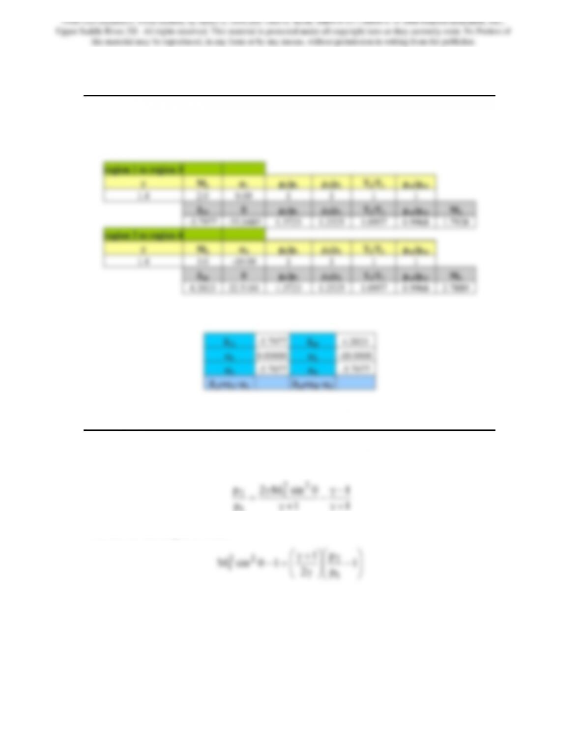
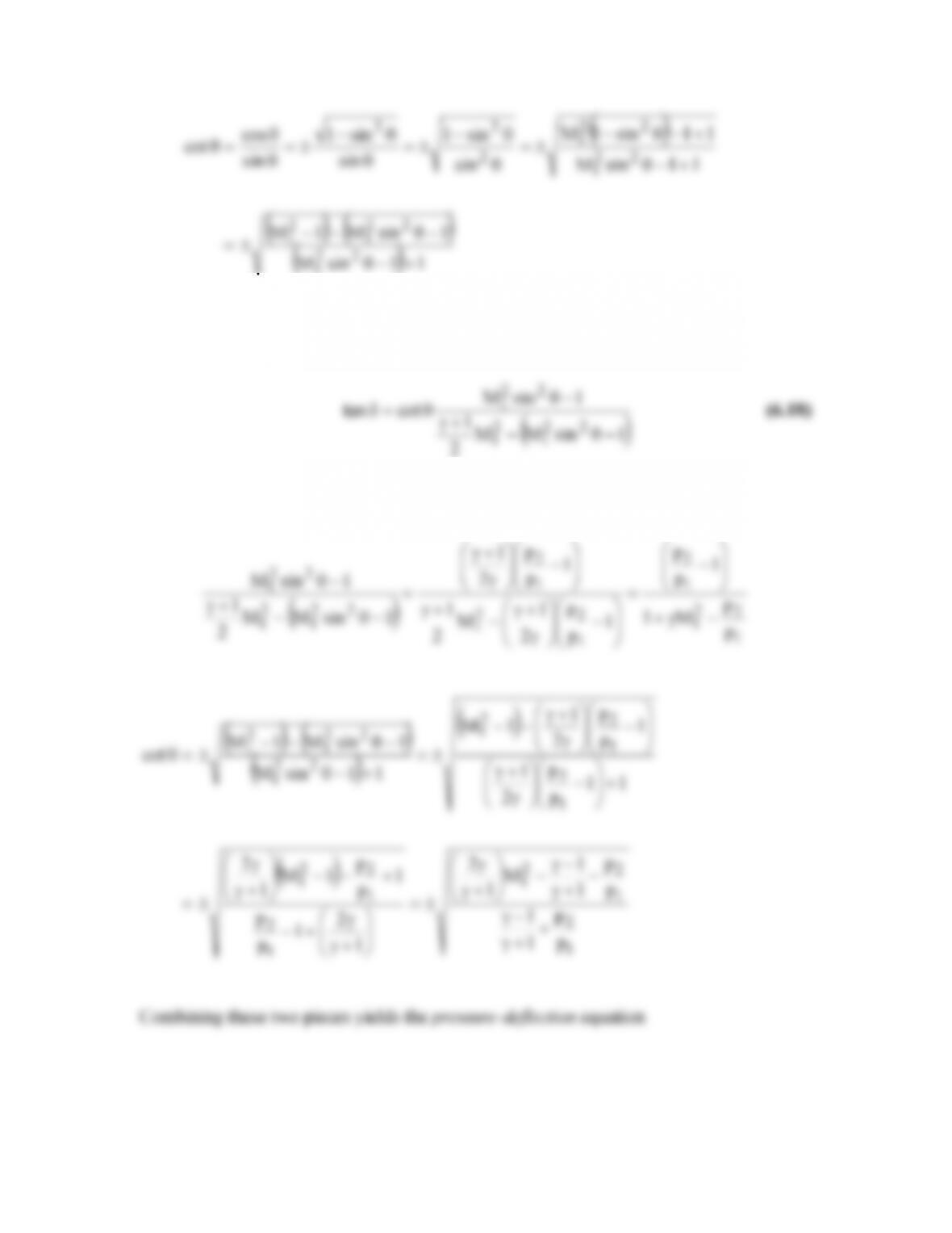
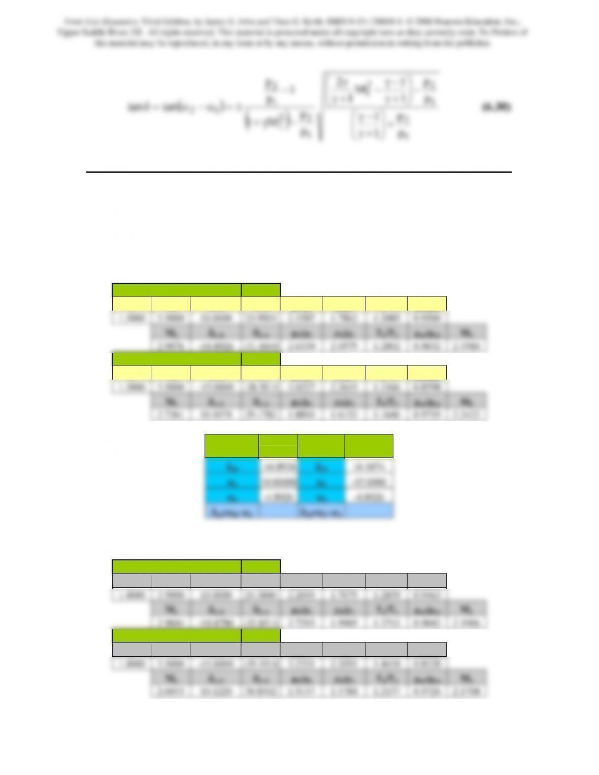
Problem 21. – Derive the pressure-deflection equation, i.e., Eq.(6.30).

The expression for the pressure ratio across an oblique shock, is given in Eq.(6.10)

1

sinM2

p

p22

1

+γ

−γ

+γ

θγ

This can be rearranged to obtain

The following identity is also used in this development

this material may be reproduced, in any form or by any means, without permission in writing from the publisher.

126

(

)

()

11sinM

11sin1M

sin

sin1

sin

sin1

sin

cos

cot

1

22

1

22

1

2

22

+−θ

+−θ−

±=

θ

θ−

±=

θ

θ−

±=

θ

=θ

Now the deflection angle is connected to the shock wave angle and the upstream Mach

number by Eq.(6.18)

()

1sinMM

2

1

22

1

2

1

−θ−

+γ

Dividing the expression on the right into two pieces

2

1

2

1

2

22

2

22

1

p

1

p

1

p

2

1

1sinM

⎟

⎠

⎞

⎜

⎝

⎛−

=

⎞

⎛−

⎞

⎛

+γ

⎟

⎠

⎞

⎜

⎝

⎛−

⎟

⎠

⎞

⎜

⎝

⎛

γ

+γ

=

+γ

−θ

this material may be reproduced, in any form or by any means, without permission in writing from the publisher.

1

2

1

2

p

1

M

1

2

1

p

−

⎟

⎠

⎞

⎜

⎝

⎛

+γ

−γ

−

+γ

γ

−

Problem 22. – Repeat the computations of Example 6.8 to find the angle the slip line

makes with the horizontal for γ = 1.4 and 1.667. How does the angle vary with γ?

Results of the computations for all three specific heat ratios (1.3, 1.4 and 5/3) is as

follows:

γ = 1.3

region 1 to region 2 to region 4

γ M1 δ1−2 θ1−2 p2/p1 ρ2/ρ1 T2/T1 po2/po1

region 1 to region 3 to region 5

γ M1 δ1−3 θ1−3 p3/p1 ρ3/ρ1 T3/T1 po3/po1

Downstream

flow angles

γ = 1.4

region 1 to region 2 to region 4

γ M1 δ1−2 θ1−2 p2/p1 ρ2/ρ1 T2/T1 po2/po1

region 1 to region 3 to region 5

γ M1 δ1−3 θ1−3 p3/p1 ρ3/ρ1 T3/T1 po3/po1

this material may be reproduced, in any form or by any means, without permission in writing from the publisher.

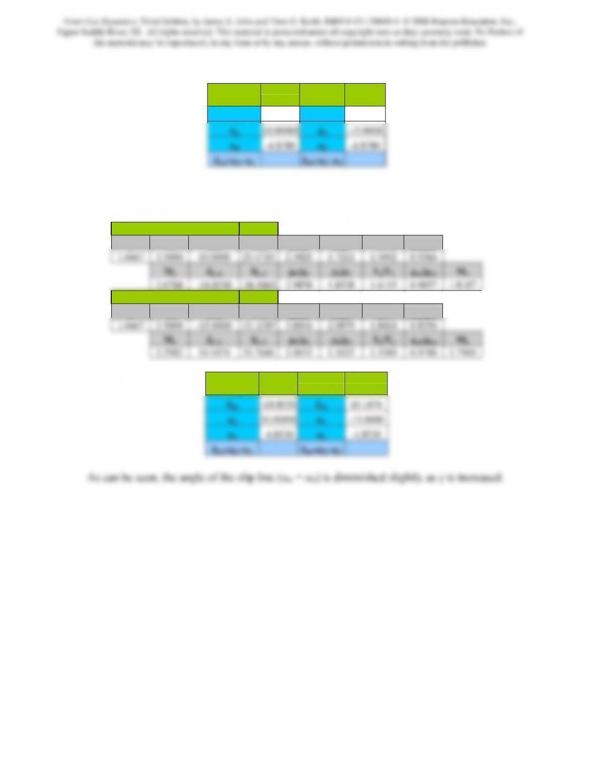
Downstream

flow angles

δ24 -14.8780 δ35 10.1220

γ = 5/3

region 1 to region 2 to region 4

γ M1 δ1−2 θ1−2 p2/p1 ρ2/ρ1 T2/T1 po2/po1

region 1 to region 3 to region 5

γ M1 δ1−3 θ1−3 p3/p1 ρ3/ρ1 T3/T1 po3/po1

Downstream

flow angles

this material may be reproduced, in any form or by any means, without permission in writing from the publisher.