978-0131206687 Chapter 15

C

Ch

ha

ap

pt

te

er

r

F

Fi

if

ft

te

ee

en

n

M

ME

EA

AS

SU

UR

RE

EM

ME

EN

NT

TS

S

I

IN

N

C

CO

OM

MP

PR

RE

ES

SS

SI

IB

BL

LE

E

F

FL

LO

OW

W

Problem 1. – A Pitot tube is placed in a uniform air flow of Mach 2.5. If the Pitot tube indicates

a pressure of 500 kPa, find the static pressure of the flow. Take γ = 1.40.

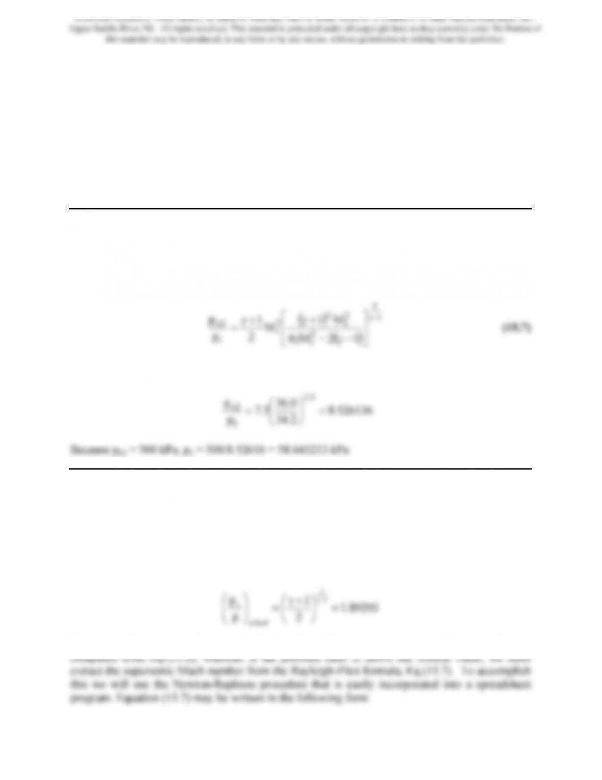
From the Rayleigh-Pitot formula, Eq. (15.7), we have

()

1

2

1

2

1

2

1

2o

12M4

M1

2

1

p

p−γ

⎥

⎦

⎤

⎢

⎣

⎡

−γ−γ

+γ

For an M1 = 2.5 and γ = 1.4, the pressure ratio is computed to be

Problem 2. – A Pitot tube is placed in a uniform helium flow. If the Pitot tube indicates a

pressure of 280 kPa and the static pressure of the flow is measured to be 20 kPa, find the Mach

number. Take γ = 1.40.

This is the same type of problem as in Example 15.1. Thus, many of the same steps are repeated

herein. The first step is to compute the critical pressure ratio, i.e., Eq.(15.1) at M = 1 and γ = 1.4,

If the actual pressure ratio po2/p1 is below the critical value, a subsonic Mach number is

339

this material may be reproduced, in any form or by any means, without permission in writing from the publisher.

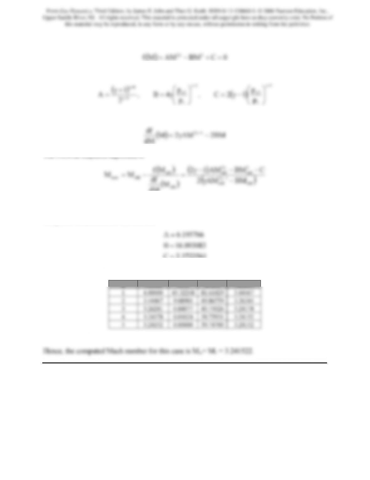
where the coefficients in this expression are

1

p

2

−γ−γ

−γ

+γ

⎟

⎠

⎜

⎝

⎟

⎠

⎜

⎝

The derivative of this function is

()

BM2AM2M

dM

df 12 −γ= −γ

The Netwon-Raphson algorithm is

old

dM

For this case po2 = 280 kPa and p1 = 20 kPa, so the pressure ratio is 14.000, which is well above

the critical pressure ratio for the given ratio of specific heats. It should be noted that the

computed coefficients for this case are

3722561.2C

195766.6A

=

The results of the iterative computations are presented in following table

n M(old) f(M) df/dM M(new)

Rayleigh-Pitot formula computations

Problem 3. – A uniform flow of air at Mach 2.0 passes over an insulated wall. The static

temperature and pressure in the free stream outside the boundary layer are, respectively, 250 K

and 20 kPa. Determine the free-stream stagnation temperature, adiabatic wall temperature, and

static pressure at the wall surface. Take γ = 1.40.

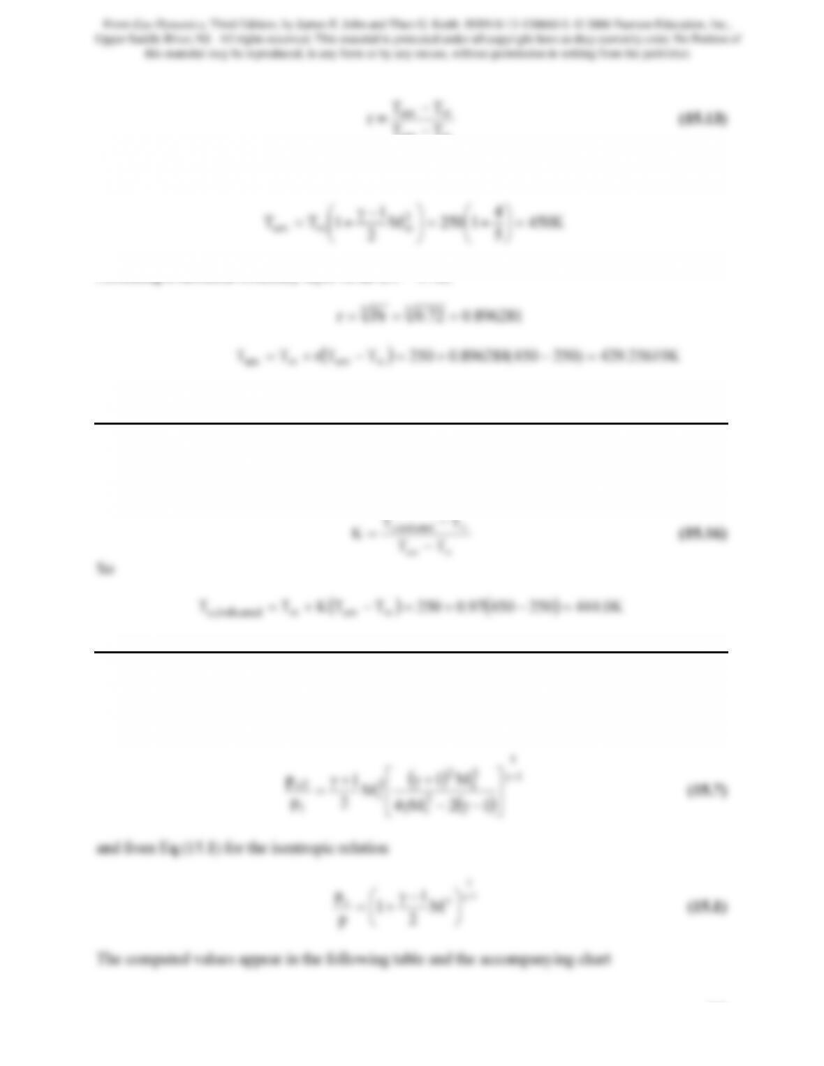
From Eq.(15.13) we have

340

this material may be reproduced, in any form or by any means, without permission in writing from the publisher.

∞∞

−

o

Since T∞ = 250K and M∞ = 2.0

5

2

o=

⎠

⎝

⎠

⎝

Assuming a turbulent boundary layer of air (Pr = 0.72)

The static pressure at the wall is the same as the free stream static pressure: 20kPa

Problem 4. – A total temperature probe is inserted into the flow of Problem 3. If the probe has K

[see Eq.(15.16)] equal to 0.97, what temperature will be indicated by the probe?

From Eq.(15.16)

∞

−

TT

indicated,o (15.16)

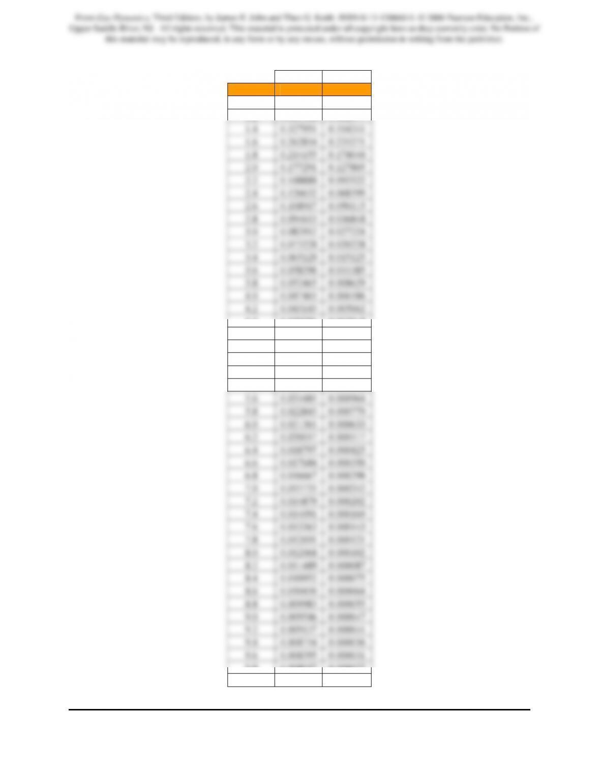
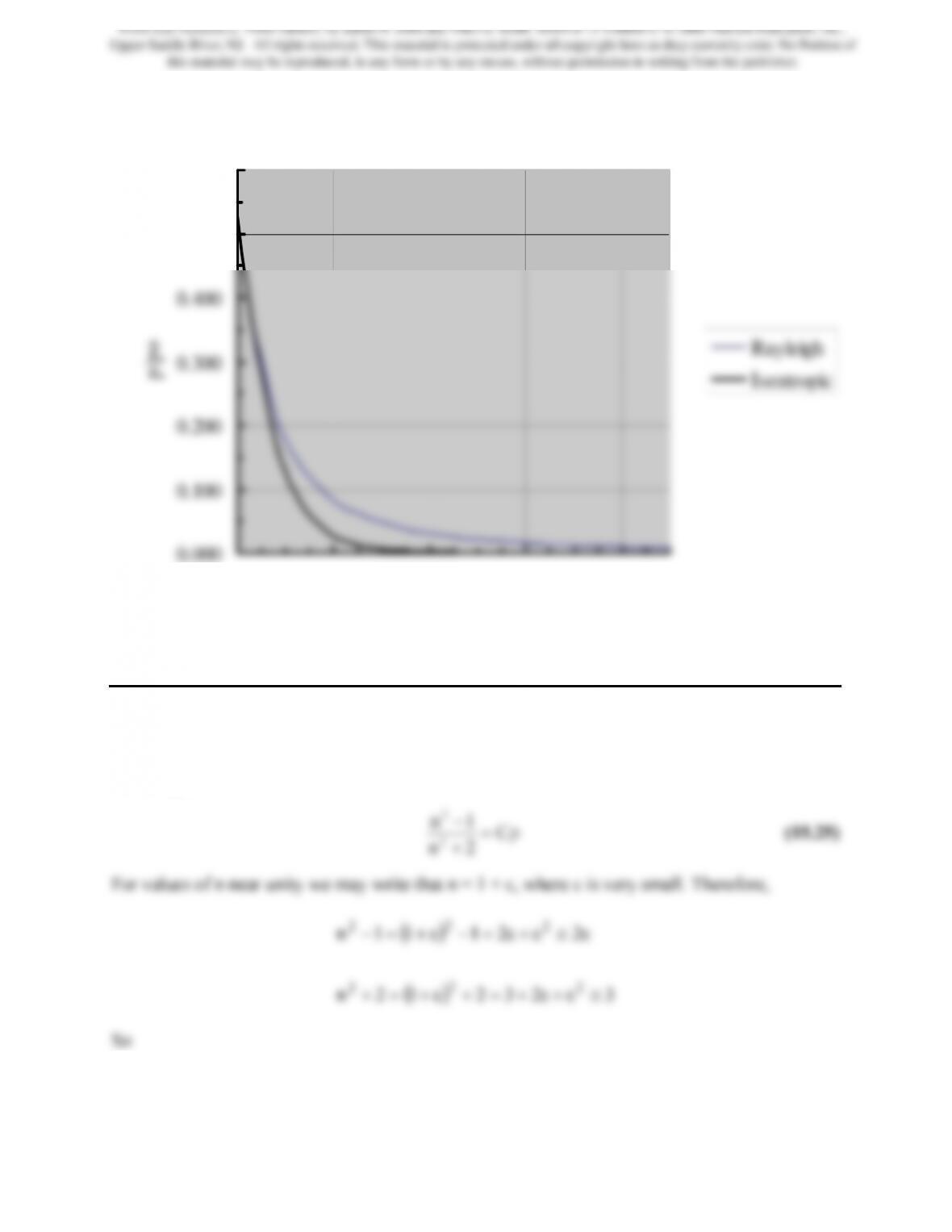
Problem 5. – Sketch a plot of p/po versus M for isentropic flow. On the same coordinates, plot

p∞/pPitot versus M∞. Take γ = 1.40.

Values are computed for a range of Mach numbers from Eq.(15.7) for the Raleigh Pitot formula

()

1

2

1

2

2o

M1

1

p−γ

⎤

⎡

+γ

341

this material may be reproduced, in any form or by any means, without permission in writing from the publisher.

Rayleigh isentropic

M1 p1/po2 p/po

1.0 0.528282 0.528282

1.2 0.415368 0.412377

4.4 0.039381 0.003918

4.6 0.036088 0.003053

4.8 0.033189 0.002394

5.0 0.030625 0.001890

5.2 0.028345 0.001501

5.4 0.026310 0.001200

9.8 0.008057 0.000027

10.0 0.007739 0.000024

342

this material may be reproduced, in any form or by any means, without permission in writing from the publisher.

0.000

0.100

0.200

0.300

0.400

0.500

0.600

1.0 3.0 5.0 7.0 9.0

M1

Rayleigh

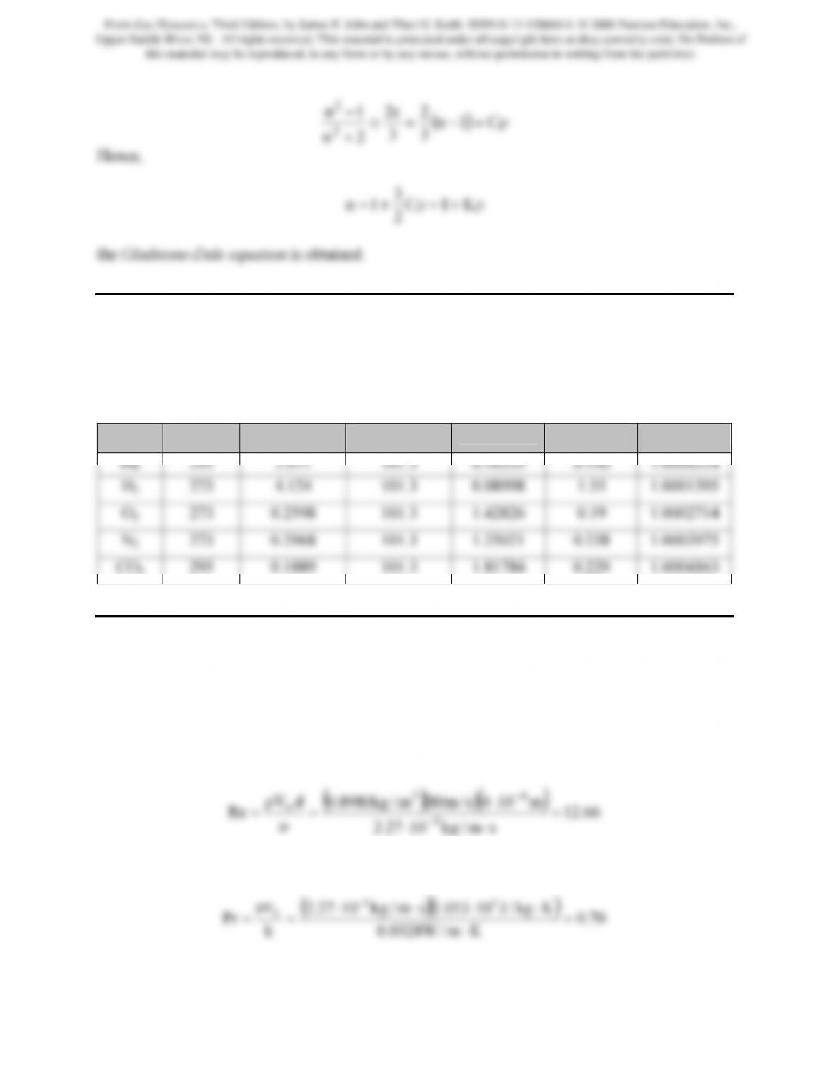
Problem 6. – Derive the Gladstone-Dale relation, Eq.(15.26), from the Lorenz-Lorentz relation,

Eq.(15.25).

From Eq.(15.25) we have

343

this material may be reproduced, in any form or by any means, without permission in writing from the publisher.

ε

−C1n

2

1n

2

Problem 7. – Compute the index of refraction at atmospheric pressure for the gases contained in

Table 15.1 for the given Gladstone-Dale constants and temperatures.

To use the Gladstone-Dale equation, we must first compute the density of each gas assuming

each behaves as a perfect gas

Gas T (K) R (kJ/kg·K) p (kPa) ρ (m3/kg) K (cm3/g) n

Problem 8. – The wire of a hot wire anemometer is placed to an air flow at atmospheric pressure

with a temperature of 30°C and a velocity of 80 m/s. The wire is heated to a constant temperature

of 210°C. The diameter of the wire is 4 µm and its length is 2 mm. Determine the electric current

in the wire. The air properties at the mean film temperature are: ρ = 0.898 kg/m3, µ = 2.27⋅10-5

kg/m⋅s, k=0.0328 W/m⋅K, and cp=1.013 kJ/kg⋅K. The resistivity of the wire is 0.22 µΩ⋅m.

The Reynolds number is:

66.12

sm/kg1027.2

Re 5

⋅⋅

=

µ

=−

The Prandtl number is:

35

−

344

this material may be reproduced, in any form or by any means, without permission in writing from the publisher.

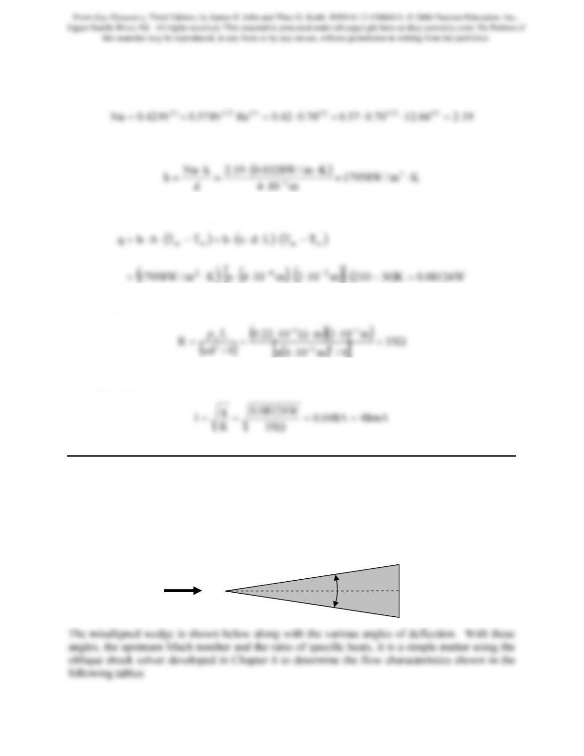
With Prandtl and Reynolds numbers we can determine the Nusselt number from Kramers

correlation, Eq.(15.23):

The heat transfer coefficient can then be calculated as:

m104

d

6⋅=

⋅

The heat loss from the wire is given by:

()()()

[]

()

W08124.0K30210m102m104Km/W17958

362

=−⋅⋅⋅⋅⋅π⋅⋅=

−−

The resistance of the wire is:

()

[ ]

Ω=

⋅π

=

π

=−

35

4/m104

4/d

R2

6

2

Consequently, the electric current in the wire is:

35

R

Ω

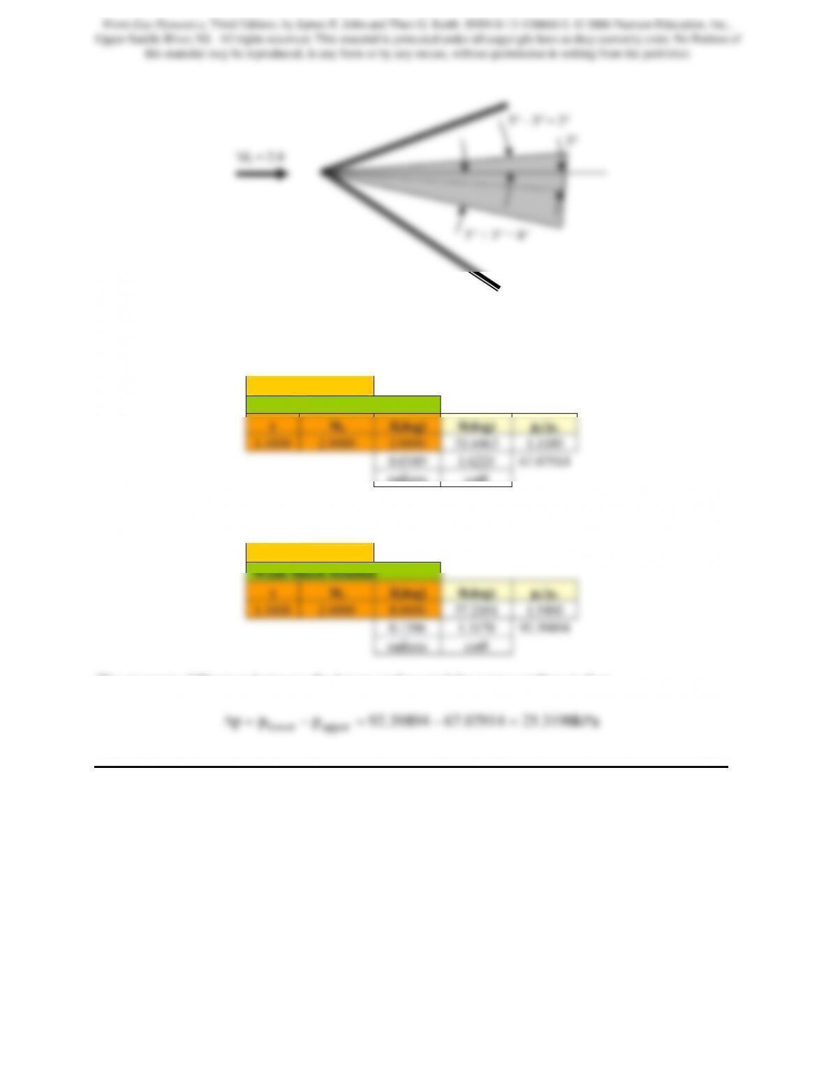
Problem 9. – A symmetrical wedge of 10° total included angle is placed in a uniform Mach 2.0

flow of static pressure of 60 kPa. If the axis of the wedge is misaligned with the flow direction

by 3°, determine the static pressure difference between the top and bottom surfaces of the wedge.

Take γ = 1.40

The symmetrical wedge is shown as follows

10°

M1 = 2.0

345

this material may be reproduced, in any form or by any means, without permission in writing from the publisher.

Upper Surface

Given: M1 and δ

Weak Shock Solution

radians

cotθ

Lower Surface

Given: M1 and δ

The pressure difference between the lower surface and the upper surface is then

Problem 10. – The temperature of the wire of an anemometer placed perpendicular to an air flow

of 20°C is 100°C. The wire dissipates 20 mW of heat to the flow. The diameter of the wire is 3

µm and the length 1 mm. What is the velocity of the flow? The properties of the air at the mean

temperature between fluid and the wire are: ρ = 1.0595 kg/m3, cp = 1.009 kJ/kg, k = 0.0285

W/m⋅K, and µ = 2⋅10-5 kg/m⋅s.

The heat transfer coefficient is:

5° + 3° = 8°

346

this material may be reproduced, in any form or by any means, without permission in writing from the publisher.

()()

()

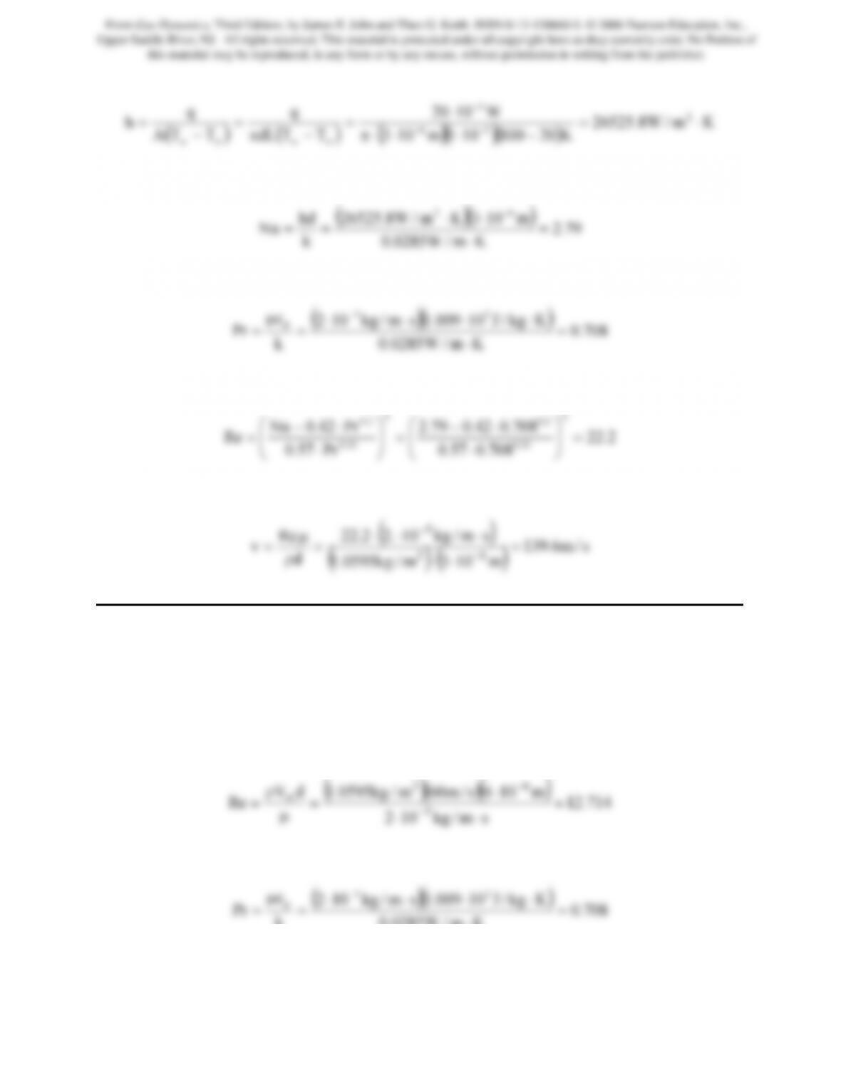
Km/W8.26525

K20100101m103

W1020

TTdL

q

TTA

q

h2

36

3

ww

⋅=

−⋅⋅⋅π

⋅

=

−π

=

−

=−−

−

∞∞

The Nusselt number is computed from:

Km/W0285.0

k

62

⋅

−

The Prandtl number is:

Km/W0285.0

k

⋅

Therefore, the Reynolds number is determined from Kramers correlation, Eq.(15.26):

708.057.0

708.042.079.2

Pr57.0

Pr42.0Nu

2

33.0

2.0

2

33.0

2.0

⎟

⎠

⎞

⎜

⎝

⎛

⋅

⋅−

⎟

⎠

⎞

⎜

⎝

⎛

⋅

⋅−

The velocity of the flow is therefore:

()()

m103m/kg0595.1

d

⋅⋅

ρ

Problem 11. – The sensing element of a hot wire anemometer is a platinum wire 4 µm diameter

and 2 mm length. The wire is placed perpendicular to an air flow at atmospheric pressure with a

temperature of 20°C and a velocity of 60 m/s. If the temperature of the wire is 100°C, determine

the power dissipated by the wire. The properties of the air at the mean film temperature are:

ρ = 1.0595 kg/m3, cp = 1.009 kJ/kg⋅K, k = 0.0285 W/m⋅K, µ = 2⋅10-5 kg/m⋅s.

The Reynolds number is:

714.12

sm/kg102

Re 5

63 =

⋅⋅

=

µ

=−

−

The Prandtl number is:

Km/W0285.0

k

⋅

The Nusselt number can be computed using the Kramers correlation, Eq.(15.23):

347

this material may be reproduced, in any form or by any means, without permission in writing from the publisher.

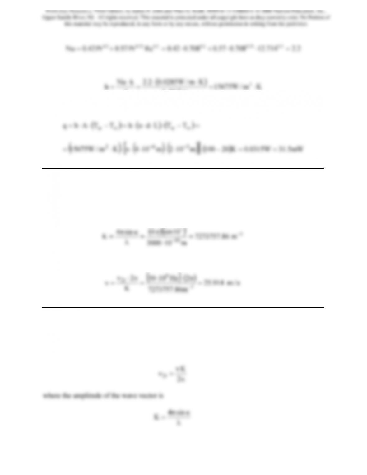
The heat transfer coefficient is:

m104

d

6⋅=

⋅

The heat loss from the wire is:

()()()

[]

()

mW5.31W0315.0K20100m102m104Km/W15675

362

==−⋅⋅⋅⋅⋅π⋅⋅=

−−

Problem 12. – A dual beam LDV-system with a wavelength of 3000Å and a 20o angle between

the intersecting beams records a difference of 30MHz between the two Doppler shifts. What is

the velocity of the flow-field?

The amplitude of the wave vector is

( )

1

10 m86.7273757

m103000

10sin4

sin4

−=

⋅

π

λ

κπ

o

The velocity of the seeding particle (assumed equal to the velocity of the flow) is

( )

2Hz1030

2

6

D=

π⋅⋅

π⋅ν

Problem 13. – What is the minimum frequency that a dual beam LDV system has to have in

order to measure a 1000 m/s velocity with a 5000 Å laser with a 5o angle between the beams?

Explain using both theoretical explanations of the LVD instrument.

Using the Doppler shift explanation: the frequency difference between the two Doppler shifts is

348

this material may be reproduced, in any form or by any means, without permission in writing from the publisher.

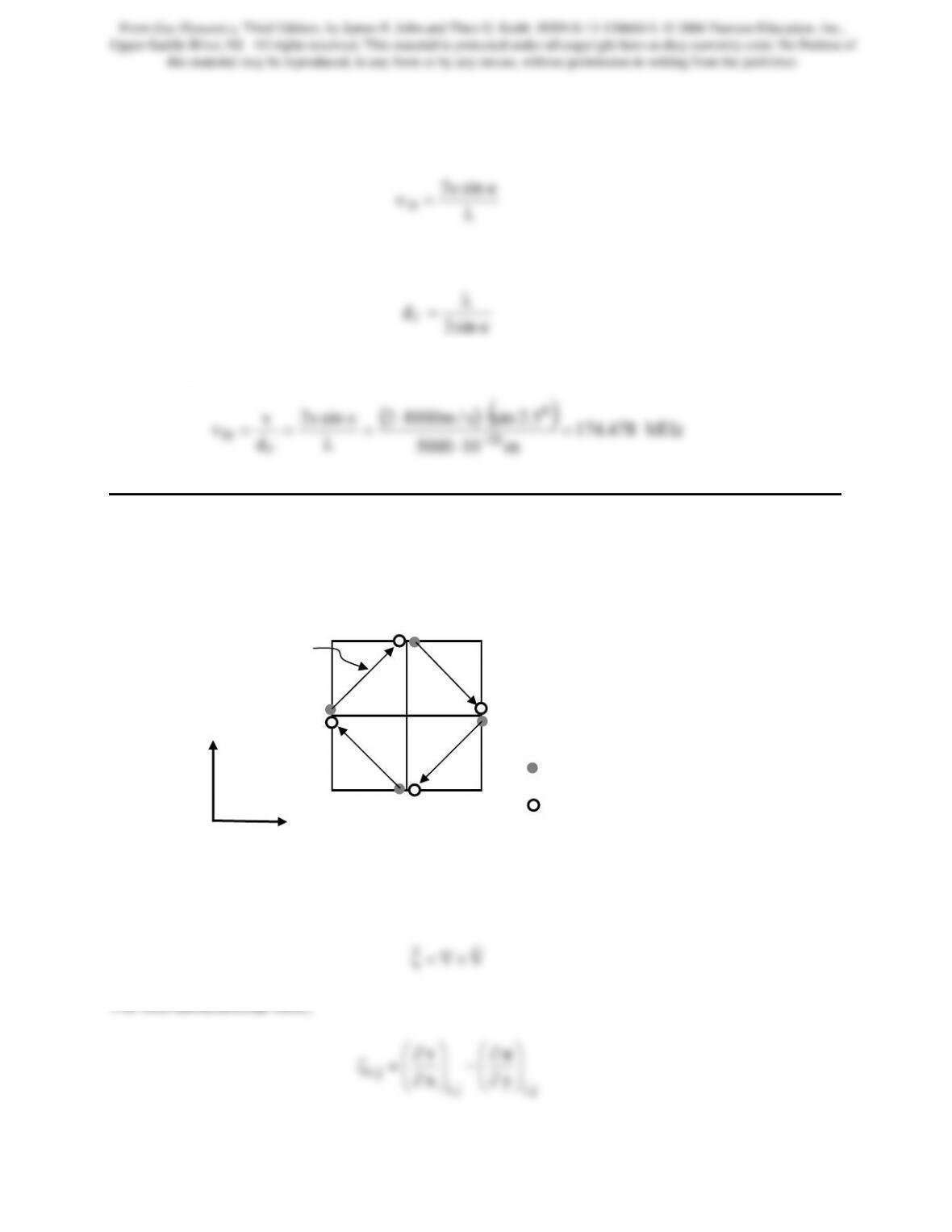
so the frequency to detect is

Alternately, using the fringe model: the fringe spacing distance is

λ

so the frequency to detect can be determined, as above, from,

m105000

d

10

f

D=

⋅

λ

Problem 14. – Determine the vorticity of the flowfield based on the double-exposed PIV

photograph shown Figure P15.14. The interval between the two exposures is ∆t = 0.001s. The

grid-size equals 1mm in both directions.

Figure P15.14

The vorticity of the flow is defined as

V

j,ij,i

j,i y

x

⎠

⎜

⎝

∂

⎟

⎠

⎜

⎝

∂

First exposure (t = 0)

Second exposure (t = ∆t)

(i, j+1)

(i, j) (i+1, j)

(i-1, j)

(i, j-1)

j,1i

V−

r

x

y

349

this material may be reproduced, in any form or by any means, without permission in writing from the publisher.

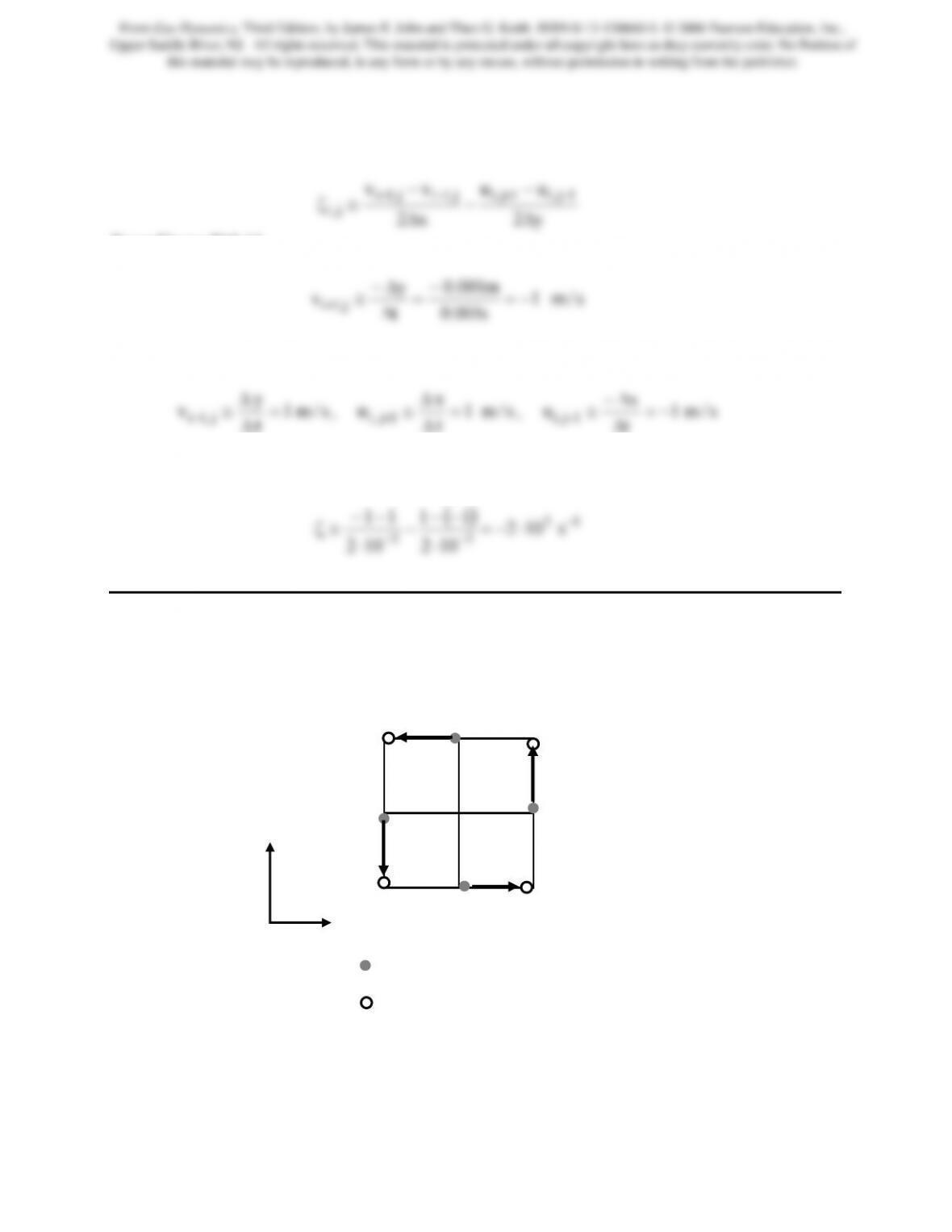
The vorticity can be numerically approximated using central differences as

x2

j,i ∆

∆

From Figure P15.14

s001.0

m001.0

t

y

−

∆

∆−

Similarly,

t

∆

t

∆

t

∆

Hence, the vorticity is

( )

13

11

11 −

−−

Problem 15. – A double–exposed PIV photograph contains the flowfield illustrated in Figure

P15.15. Show that if the grid-size is equal in the x and y directions, i.e., ∆x = ∆y, the vorticity at

(i,j) is only dependent upon the time interval ∆t between the two exposures.

Figure P15.15

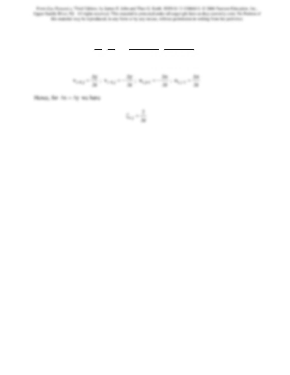
The vorticity can be numerically calculated from

(i, j+1)

(i, j) (i+1, j)

(i-1, j)

(i, j-1)

First exposure (t = 0)

Second exposure (t=∆t)

x

y

350

this material may be reproduced, in any form or by any means, without permission in writing from the publisher.

y2

uu

x2

vv

y

u

x

v1j,i1j,ij,1ij,1i

j,i

j,i ∆

−

∆

−

≅

⎟

⎠

⎞

⎜

⎝

⎛

∂

−

∂

=ζ −+−+

Now,

351

this material may be reproduced, in any form or by any means, without permission in writing from the publisher.