978-0131206687 Chapter 14 Part 3

325

.

Point Area A/A*

M

(Exact Solution)

M

(MOC) % Error

4 A4 10.7188 4.00 4.0000

11 1.0637A4 12.3051 4.1558 4.1557 -0.0014

18 1.1334A4 14.1642 4.3172 4.3207 0.0799

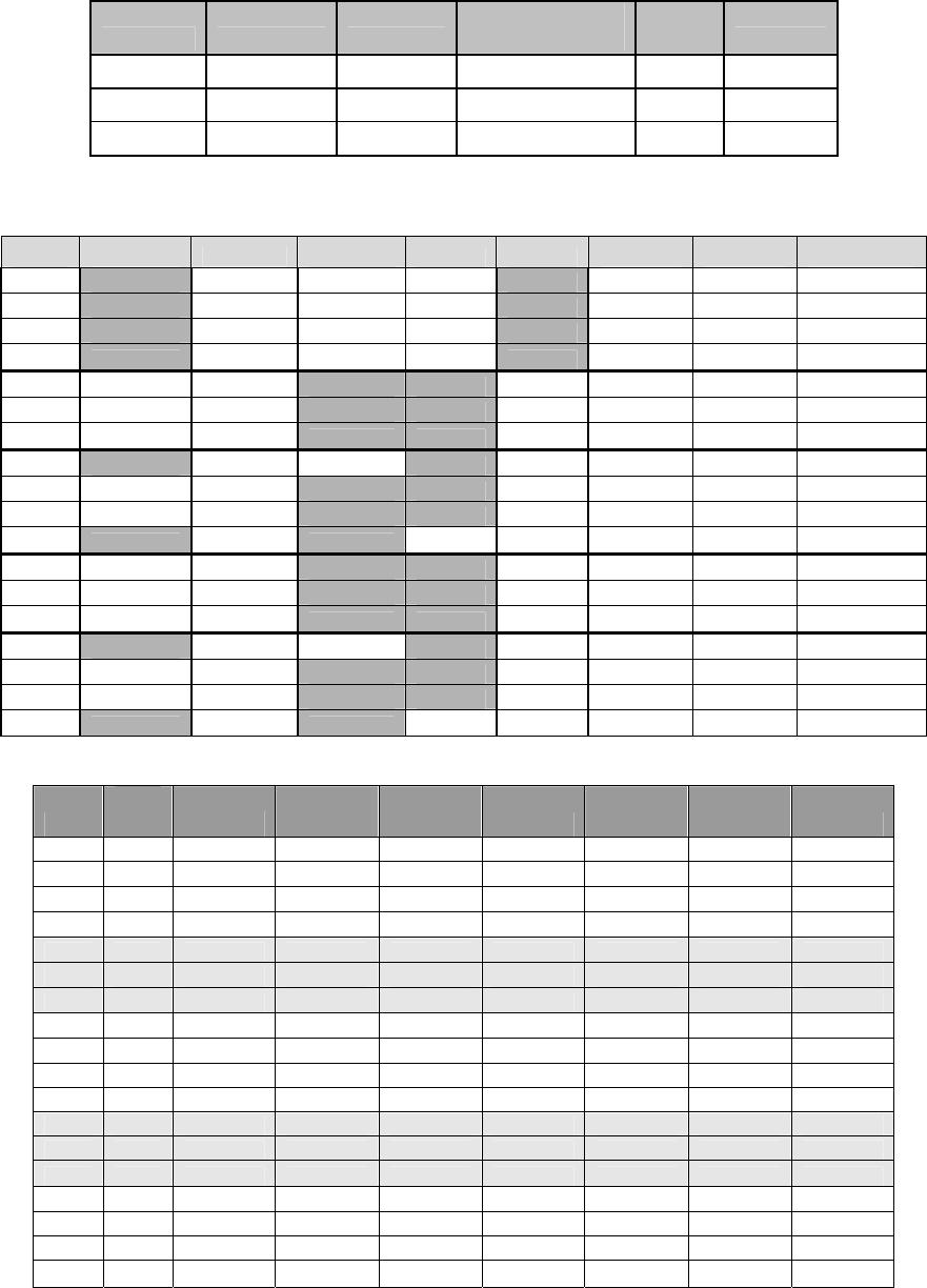
(c) Minitial = 2.0, total wedge angle of 24˚ and γ = 1.4

point α deg ν C(+)I C(-)II M µ α + µ α − µ

1 12.00 26.3798 38.3798 14.3798 2.0000 30.0000 42.0000 -18.0000

2 8.00 26.3798 34.3798 18.3798 2.0000 30.0000 38.0000 -22.0000

3 4.00 26.3798 30.3798 22.3798 2.0000 30.0000 34.0000 -26.0000

4 0.00 26.3798 26.3798 26.3798 2.0000 30.0000 30.0000 -30.0000

5 10.00 28.3798 38.3798 18.3798 2.0733 28.8370 38.8370 -18.8370

6 6.00 28.3798 34.3798 22.3798 2.0733 28.8370 34.8370 -22.8370

7 2.00 28.3798 30.3798 26.3798 2.0733 28.8370 30.8370 -26.8370

8 12.00 30.3798 42.3798 18.3798 2.1483 27.7419 39.7419 -15.7419

9 8.00 30.3798 38.3798 22.3798 2.1483 27.7419 35.7419 -19.7419

10 4.00 30.3798 34.3798 26.3798 2.1483 27.7419 31.7419 -23.7419

11 0.00 30.3798 30.3798 30.3798 2.1483 27.7419 27.7419 -27.7419

12 10.00 32.3798 42.3798 22.3798 2.2251 26.7068 36.7068 -16.7068

13 6.00 32.3798 38.3798 26.3798 2.2251 26.7068 32.7068 -20.7068

14 2.00 32.3798 34.3798 30.3798 2.2251 26.7068 28.7068 -24.7068

15 12.00 34.3798 46.3798 22.3798 2.3039 25.7250 37.7250 -13.7250

16 8.00 34.3798 42.3798 26.3798 2.3039 25.7250 33.7250 -17.7250

17 4.00 34.3798 38.3798 30.3798 2.3039 25.7250 29.7250 -21.7250

18 0.00 34.3798 34.3798 34.3798 2.3039 25.7250 25.7250 -25.7250

point

α

deg µ α + µ α − µ mI mII x y

1 12 30 42 -18 4.7046 1.0000

2 8 30 38 -22 4.7629 0.6694

3 4 30 34 -26 4.7980 0.3355

4 0 30 30 -30 4.8097 0.0000

5 10 28.8370 38.8370 -18.8370 -0.3330 0.7931 5.0393 0.8886

6 6 28.8370 34.8370 -22.8370 -0.4125 0.6852 5.0890 0.5349

7 2 28.8370 30.8370 -26.8370 -0.4968 0.5871 5.1139 0.1786

8 12 27.7419 39.7419 -15.7419 0.2126 0.8182 5.3407 1.1352

9 8 27.7419 35.7419 -19.7419 -0.3806 0.6454 5.4153 0.7455

10 4 27.7419 31.7419 -23.7419 -0.4628 0.7078 5.4084 0.3870

11 0 27.7419 27.7419 -27.7419 -0.5159 0.0000 5.4600 0.0000

12 10 26.7068 36.7068 -16.7068 -0.2910 0.7325 5.7749 1.0089

13 6 26.7068 32.7068 -20.7068 -0.3684 0.6303 5.7698 0.6148

14 2 26.7068 28.7068 -24.7068 -0.4499 0.5367 5.8288 0.1979

15 12 25.7250 37.7250 -13.7250 0.2126 0.7595 6.1746 1.3124

16 8 25.7250 33.7250 -17.7250 -0.3099 0.6548 6.1799 0.8834

17 4 25.7250 29.7250 -21.7250 -0.3882 0.5592 6.2447 0.4305

18 0 25.7250 25.7250 -25.7250 -0.4709 0.0000 6.2490 0.0000

this material may be reproduced, in any form or by any means, without permission in writing from the publisher.

326

.

Point Area A/A*

M

(Exact Solution)

M

(MOC) % Error

4 A4 1.6875 2.00 2.0000

11 1.0637A4 1.9157 2.1483 2.1483 -0.0004

18 1.1334A4 2.1925 2.2997 2.3039 0.1827

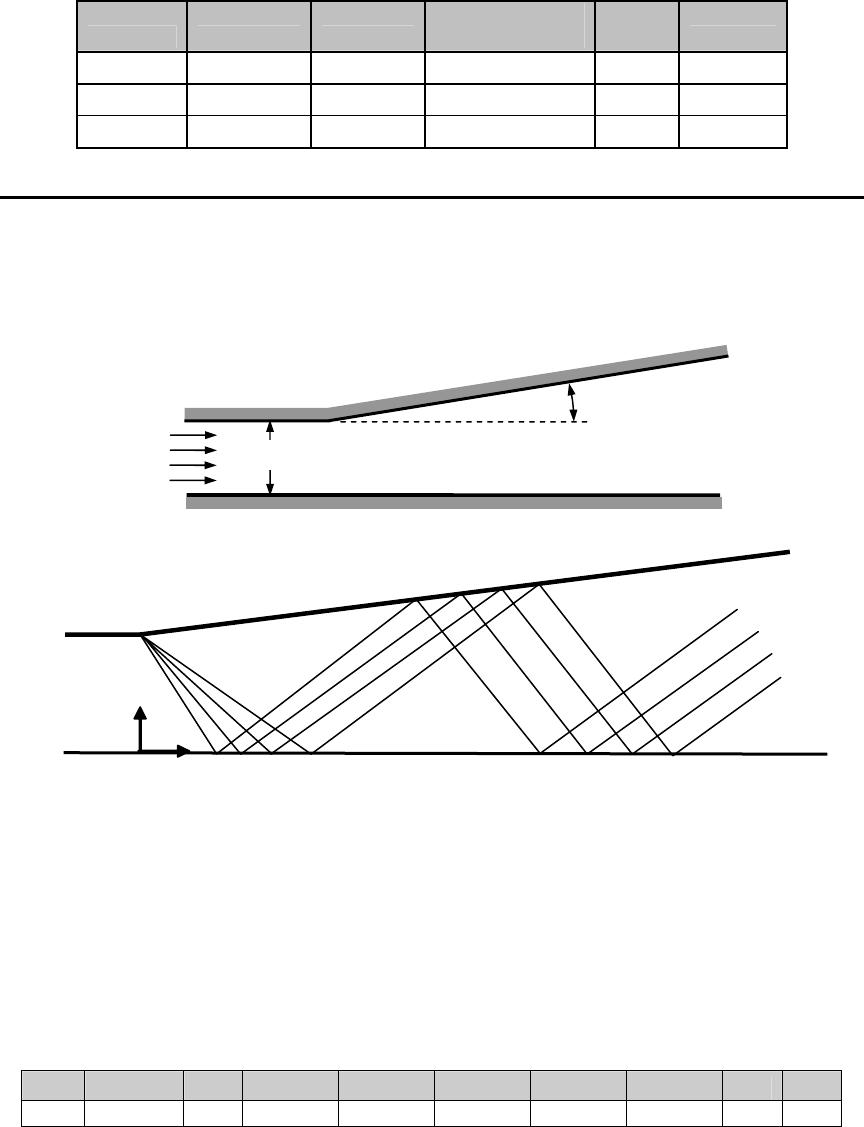
Problem 16. – A supersonic flow at Mach 1.8 and γ = 1.4 enters the channel shown in

Figure P14.16(a). Using the point-to-point method of characteristics, determine the Mach

number distribution throughout the flow for the pattern shown in Figure P14.16(b).

(a)

(b)

Figure P14.16

A spreadsheet program was constructed to solve this problem. Results of the program are

contained within the following:

Input and computed initial data-

γ γ-1/γ+1 α1 M1 wall ang turns ∆(angle) xo yo p1

1.4 0.1667 0 1.8 8 4 2 0 0.1 10

Results of calculations-

cm10

kPa10p

8.1M

1

=

8˚

1

0

5

6

10

11

22

23

4

17

24

26

15

16

20

21

25

28

30

27

29

3

7

28

9

12

13

14

18

19

x

y

this material may be reproduced, in any form or by any means, without permission in writing from the publisher.

327

Method: Point-to–

Point

Note:

a shaded cell contains a value that is

set

Point α ν CI =

ν+α

CII =

ν−α

M µ α + µ α − µ p/po

1 0.0 20.7251 20.7251 20.7251 1.8000 33.7490 33.7490 -33.7490 0.1740

2 2.0 22.7251 24.7251 20.7251 1.8697 32.3339 34.3339 -30.3339 0.1564

3 4.0 24.7251 28.7251 20.7251 1.9405 31.0204 35.0204 -27.0204 0.1402

4 6.0 26.7251 32.7251 20.7251 2.0125 29.7940 35.7940 -23.7940 0.1253

5 8.0 28.7251 36.7251 20.7251 2.0861 28.6433 36.6433 -20.6433 0.1117

6 0.0 24.7251 24.7251 24.7251 1.9405 31.0204 31.0204 -31.0204 0.1402

7 2.0 26.7251 28.7251 24.7251 2.0125 29.7940 31.7940 -27.7940 0.1253

8 4.0 28.7251 32.7251 24.7251 2.0861 28.6433 32.6433 -24.6433 0.1117

9 6.0 30.7251 36.7251 24.7251 2.1614 27.5591 33.5591 -21.5591 0.0993

10 8.0 32.7251 40.7251 24.7251 2.2385 26.5337 34.5337 -18.5337 0.0880

11 0.0 28.7251 28.7251 28.7251 2.0861 28.6433 28.6433 -28.6433 0.1117

12 2.0 30.7251 32.7251 28.7251 2.1614 27.5591 29.5591 -25.5591 0.0993

13 4.0 32.7251 36.7251 28.7251 2.2385 26.5337 30.5337 -22.5337 0.0880

14 6.0 34.7251 40.7251 28.7251 2.3177 25.5605 31.5605 -19.5605 0.0778

15 8.0 36.7251 44.7251 28.7251 2.3991 24.6340 32.6340 -16.6340 0.0685

16 0.0 32.7251 32.7251 32.7251 2.2385 26.5337 26.5337 -26.5337 0.0880

17 2.0 34.7251 36.7251 32.7251 2.3177 25.5605 27.5605 -23.5605 0.0778

18 4.0 36.7251 40.7251 32.7251 2.3991 24.6340 28.6340 -20.6340 0.0685

19 6.0 38.7251 44.7251 32.7251 2.4830 23.7497 29.7497 -17.7497 0.0601

20 8.0 40.7251 48.7251 32.7251 2.5695 22.9035 30.9035 -14.9035 0.0525

21 0.0 36.7251 36.7251 36.7251 2.3991 24.6340 24.6340 -24.6340 0.0685

22 2.0 38.7251 40.7251 36.7251 2.4830 23.7497 25.7497 -21.7497 0.0601

23 4.0 40.7251 44.7251 36.7251 2.5695 22.9035 26.9035 -18.9035 0.0525

24 6.0 42.7251 48.7251 36.7251 2.6589 22.0918 28.0918 -16.0918 0.0458

25 0.0 40.7251 40.7251 40.7251 2.5695 22.9035 22.9035 -22.9035 0.0525

26 2.0 42.7251 44.7251 40.7251 2.6589 22.0918 24.0918 -20.0918 0.0458

27 4.0 44.7251 48.7251 40.7251 2.7515 21.3117 25.3117 -17.3117 0.0397

28 0.0 44.7251 44.7251 44.7251 2.7515 21.3117 21.3117 -21.3117 0.0397

29 2.0 46.7251 48.7251 44.7251 2.8474 20.5605 22.5605 -18.5605 0.0343

30 0.0 48.7251 48.7251 48.7251 2.9470 19.8357 19.8357 -19.8357 0.0295

Problem 17. –The values of the flow angle, α, the Mach angle, µ, and the angles of the

characteristics, α ± µ, for all points of the previous problem are shown in Table P14.17.

Compute the slopes mI and mII and the x,y coordinates for each of the points.

The table below contains the computed data. The Mach angles were computed in the

previous problem from the determined Mach number.

this material may be reproduced, in any form or by any means, without permission in writing from the publisher.

328

Point µ α + µ α − µ mI mII x y

1 33.7490 33.7490 -33.7490 -0.6682 0.6682 0.1497 0.0000

2 32.3339 34.3339 -30.3339 -0.5851 0.6756 0.1595 0.0067

3 31.0204 35.0204 -27.0204 -0.5100 0.6918 0.1695 0.0136

4 29.7940 35.7940 -23.7940 -0.4409 0.7109 0.1797 0.0208

5 28.6433 36.6433 -20.6433 0.1405 0.7324 0.3562 0.1501

6 31.0204 31.0204 -31.0204 -0.5932 0.6013 0.1707 0.0000

7 29.7940 31.7940 -27.7940 -0.5185 0.6106 0.1822 0.0070

8 28.6433 32.6433 -24.6433 -0.4498 0.6302 0.1939 0.0144

9 27.5591 33.5591 -21.5591 -0.3859 0.6519 0.3850 0.1389

10 26.5337 34.5337 -18.5337 0.1405 0.6757 0.4133 0.1581

11 28.6433 28.6433 -28.6433 -0.5366 0.5462 0.1952 0.0000

12 27.5591 29.5591 -25.5591 -0.4685 0.5566 0.2086 0.0075

13 26.5337 30.5337 -22.5337 -0.4050 0.5784 0.4149 0.1268

14 25.5605 31.5605 -19.5605 -0.3452 0.6020 0.4474 0.1463

15 24.6340 32.6340 -16.6340 0.1405 0.6272 0.4814 0.1676

16 26.5337 26.5337 -26.5337 -0.4887 0.4993 0.2239 0.0000

17 25.5605 27.5605 -23.5605 -0.4254 0.5106 0.4462 0.1135

18 24.6340 28.6340 -20.6340 -0.3659 0.5339 0.4832 0.1332

19 23.7497 29.7497 -17.7497 -0.3094 0.5587 0.5222 0.1550

20 22.9035 30.9035 -14.9035 0.1405 0.5850 0.5635 0.1792

21 24.6340 24.6340 -24.6340 -0.4473 0.4586 0.7000 0.0000

22 23.7497 25.7497 -21.7497 -0.3877 0.4704 0.7573 0.0270

23 22.9035 26.9035 -18.9035 -0.3312 0.4948 0.8180 0.0570

24 22.0918 28.0918 -16.0918 -0.2773 0.5205 0.8827 0.0907

25 22.9035 22.9035 -22.9035 -0.4107 0.4225 0.8229 0.0000

26 22.0918 24.0918 -20.0918 -0.3541 0.4348 0.8930 0.0305

27 21.3117 25.3117 -17.3117 -0.3000 0.4600 0.9682 0.0650

28 21.3117 21.3117 -21.3117 -0.3779 0.3901 0.9736 0.0000

29 20.5605 22.5605 -18.5605 -0.3237 0.4027 1.0608 0.0351

30 19.8357 19.8357 -19.8357 -0.3482 0.3607 1.1615 0.0000

Table P14.17

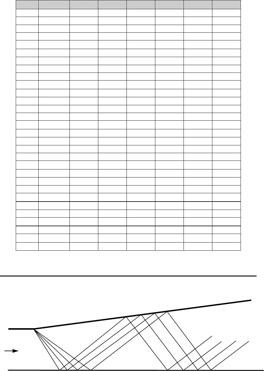
Problem 18. –Repeat Problem 14.16 using the region-to-region method for the regions

shown in Figure P14.18.

Figure P14.18

1

5

6 11

4

17

15

16

20

22 23 24

26

21

25

28

30

27

29

3

7

2 8

9

12

13

14

18

19

10

this material may be reproduced, in any form or by any means, without permission in writing from the publisher.

329

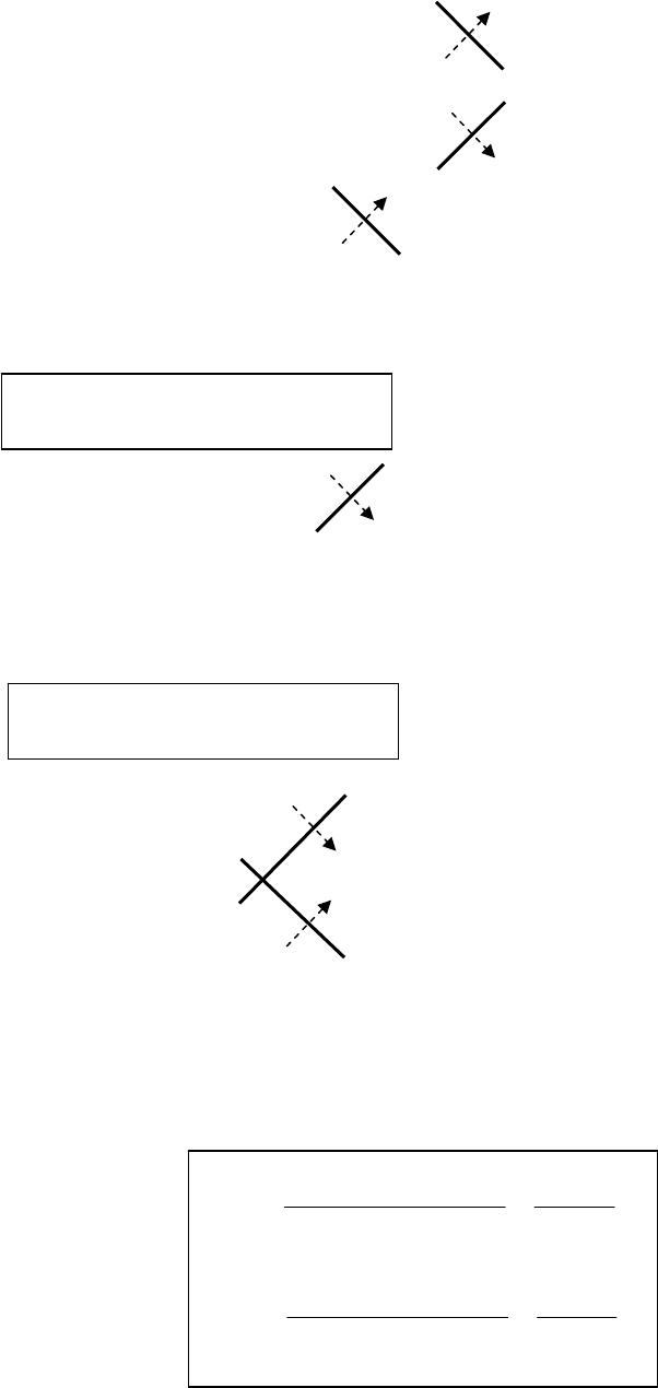
Region-to-Region Methodology:

crossing a type I characteristic: ν + α = I ∆ν = ∆α

crossing a type II characteristic: ν – α = II ∆ν = –∆α

Given: α1, ν1, and α2 Find: ν2

∆ν = ∆α

or

ν2 – ν1 = α2 – α1

so ν2 = α2 + (ν1– α1) = α2 + II1

Given: α3, ν3, and α4 Find: ν4

∆ν = −∆α

or

ν4 – ν3 = α3 – α4

so ν4 = −α4 + (ν3 + α3) = −α4 + I3

Given: α5, ν5, and α5, ν5 Find: ν7 and α7

crossing I between regions 5 and 7: ν7 – ν5 = α7 – α5 or ν7 – α7 = ν5 – α5

crossing II between regions 6 and 7: ν7 – ν6 = −(α7 – α6) or ν7 + α7 = ν6 + α6

solving these two equations simultaneously gives

()

(

)

()()

2

III

2

III

2

565566

7

565566

7

−

=

α−ν−α+ν

=α

+

=

α

−

ν

+

α

+

ν

=ν

3 4

5

7

I

6

II

1 2

this material may be reproduced, in any form or by any means, without permission in writing from the publisher.

330

Method: Region-to–

Region

Region α ν I = ν+α II = ν−α M µ α + µ α − µ

1 0.0 20.7251 20.7251 20.7251 1.8000 33.7490 33.7490 -33.7490

2 2.0 22.7251 24.7251 20.7251 1.8697 32.3339 34.3339 -30.3339

3 4.0 24.7251 28.7251 20.7251 1.9405 31.0204 35.0204 -27.0204

4 6.0 26.7251 32.7251 20.7251 2.0125 29.7940 35.7940 -23.7940

5 8.0 28.7251 36.7251 20.7251 2.0861 28.6433 36.6433 -20.6433

6 0.0 24.7251 24.7251 24.7251 1.9405 31.0204 31.0204 -31.0204

7 2.0 26.7251 28.7251 24.7251 2.0125 29.7940 31.7940 -27.7940

8 4.0 28.7251 32.7251 24.7251 2.0861 28.6433 32.6433 -24.6433

9 6.0 30.7251 36.7251 24.7251 2.1614 27.5591 33.5591 -21.5591

10 8.0 32.7251 40.7251 24.7251 2.2385 26.5337 34.5337 -18.5337

11 0.0 28.7251 28.7251 28.7251 2.0861 28.6433 28.6433 -28.6433

12 2.0 30.7251 32.7251 28.7251 2.1614 27.5591 29.5591 -25.5591

13 4.0 32.7251 36.7251 28.7251 2.2385 26.5337 30.5337 -22.5337

14 6.0 34.7251 40.7251 28.7251 2.3177 25.5605 31.5605 -19.5605

15 8.0 36.7251 44.7251 28.7251 2.3991 24.6340 32.6340 -16.6340

16 0.0 32.7251 32.7251 32.7251 2.2385 26.5337 26.5337 -26.5337

17 2.0 34.7251 36.7251 32.7251 2.3177 25.5605 27.5605 -23.5605

18 4.0 36.7251 40.7251 32.7251 2.3991 24.6340 28.6340 -20.6340

19 6.0 38.7251 44.7251 32.7251 2.4830 23.7497 29.7497 -17.7497

20 8.0 40.7251 48.7251 32.7251 2.5695 22.9035 30.9035 -14.9035

21 0.0 36.7251 36.7251 36.7251 2.3991 24.6340 24.6340 -24.6340

22 2.0 38.7251 40.7251 36.7251 2.4830 23.7497 25.7497 -21.7497

23 4.0 40.7251 44.7251 36.7251 2.5695 22.9035 26.9035 -18.9035

24 6.0 42.7251 48.7251 36.7251 2.6589 22.0918 28.0918 -16.0918

25 8.0 44.7251 52.7251 36.7251 2.7515 21.3117 29.3117 -13.3117

26 0.0 40.7251 40.7251 40.7251 2.5695 22.9035 22.9035 -22.9035

27 2.0 42.7251 44.7251 40.7251 2.6589 22.0918 24.0918 -20.0918

28 4.0 44.7251 48.7251 40.7251 2.7515 21.3117 25.3117 -17.3117

29 6.0 46.7251 52.7251 40.7251 2.8474 20.5605 26.5605 -14.5605

30 0.0 44.7251 44.7251 44.7251 2.7515 21.3117 21.3117 -21.3117

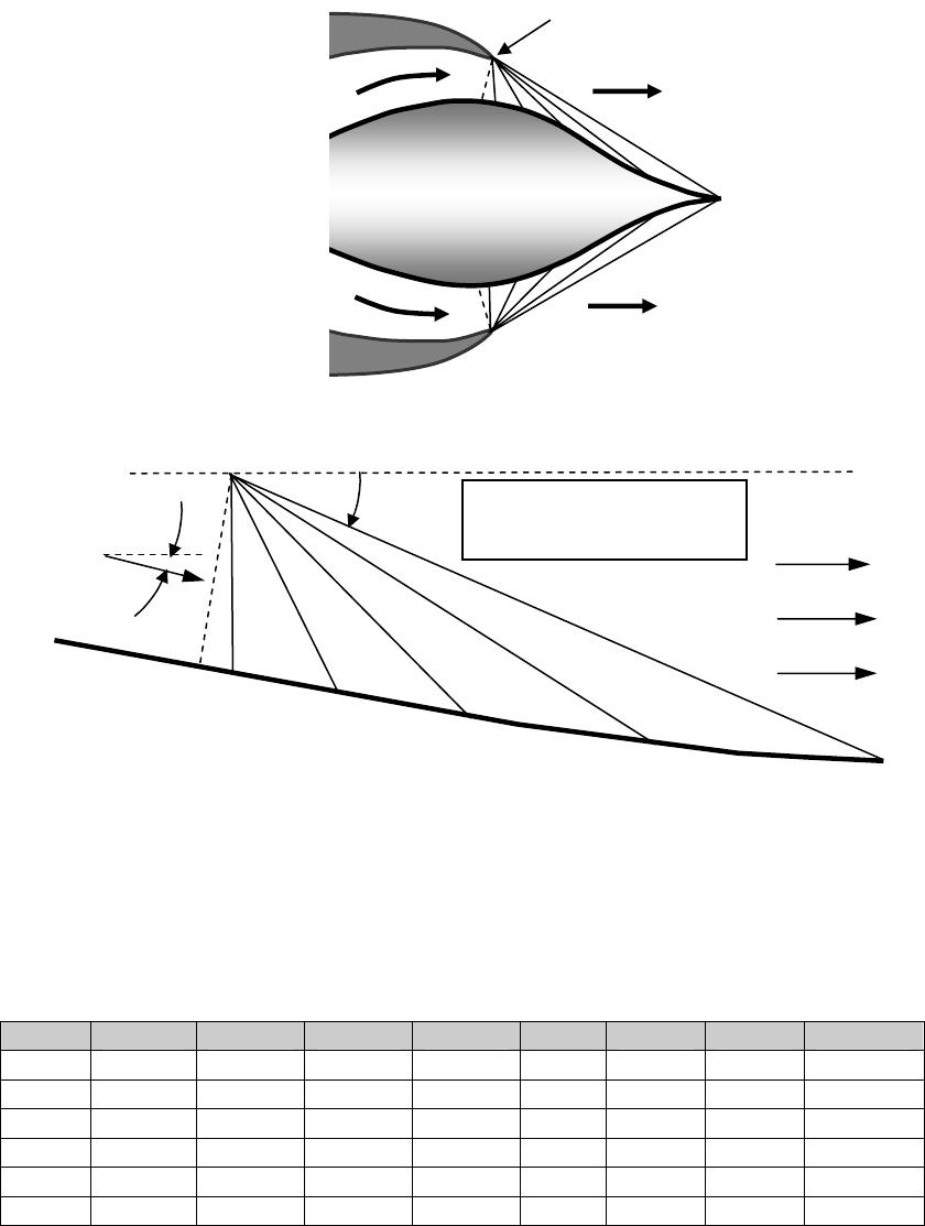
Problem 19. – Compute the supersonic flow past the curved contour of a two-

dimensional plug nozzle shown in Figure P14.19a. The contour is shaped so as to

produce cancellation of the waves incident on the plug. The nozzle is to provide a flow of

air (γ = 1.4) at Mach 1.9502856. The Mach number at the throat of the nozzle is sonic.

Use the region-to-region method for a 5 wave expansion as indicated in Figure 14.19b.

Determine the Mach number distribution and the inclinations of the characteristics.

this material may be reproduced, in any form or by any means, without permission in writing from the publisher.

331

Figure P14.19a

Figure P14.19b

In going from region 1 to region 6 we would have to cross 5 characteristics of Type I for

which ∆ν = ∆α or ν6 – ν1 = α6 – α1. Since M1 = 1 and M6 = 1.9502856, ν1 = 0 and ν6 =

25.0000, respectively. And since α6 = 0, we see that α1 = −25.0000˚. Because we are

considering the expansion to take place across 5 waves, the flow angle increases by 5˚ in

passing from region-to-region. The following table is readily established:

Region α ν I = ν+α II = ν−α M µ α + µ α − µ

1 -25.0000 0.0000 –25.0000 25.0000 1.0000 90.0000 65.0000 –115.0000

2 -20.0000 5.0000 -15.0000 25.0000 1.2565 52.7383 32.7383 -72.7383

3 -15.0000 10.0000 -5.0000 25.0000 1.4350 44.1769 29.1769 -59.1769

4 -10.0000 15.0000 5.0000 25.0000 1.6047 38.5474 28.5474 -48.5474

5 -5.0000 20.0000 15.0000 25.0000 1.7750 34.2904 29.2904 -39.2904

6 0.0000 25.0000 25.0000 25.0000 1.9503 30.8469 30.8469 -30.8469

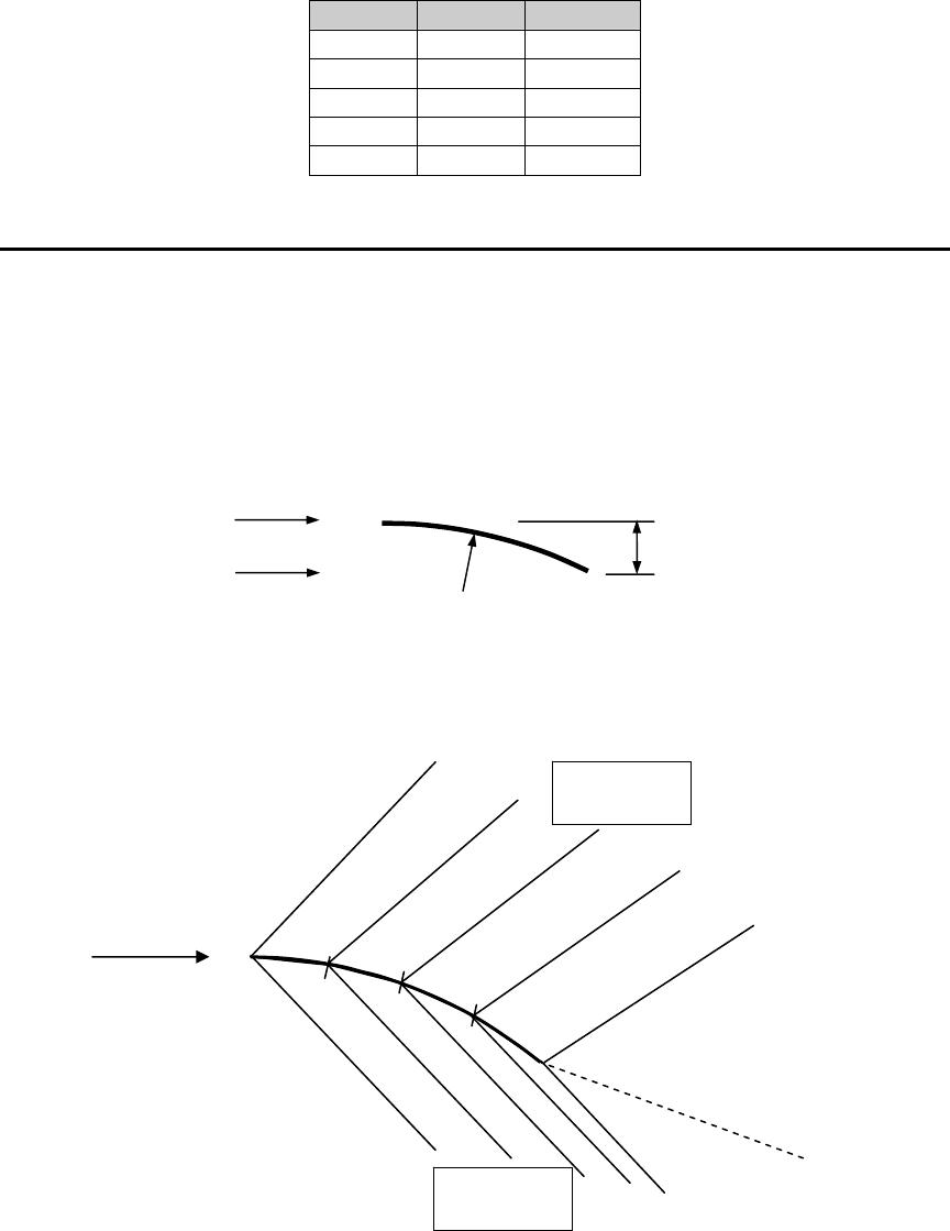
To compute the contour of the surface, we average the slopes of adjoining regions and

obtain the following

1 2 34

5 6

α1

Reference line

α

Note:

α

is CW therefore is

negative

M1 = 1

M = 1

this material may be reproduced, in any form or by any means, without permission in writing from the publisher.

332

Region Region Inclinat’n

1 2 -93.8692

2 3 -65.9576

3 4 -53.8621

4 5 -43.9189

5 6 -35.0686

Problem 20. – A thin airfoil has the form of a circular arc, as shown in Figure P14.20.

Use segregated supersonic flow along a curved surface to determine the lift and drag

coefficients for the foil at a Mach number of 1.851177. Take γ = 1.4 and divide the

circular arc into 5 linear pieces of equal length. A characteristic will emerge from each of

the corners of these lengths on both the upper and lower sides on the foil.

Figure P14.20

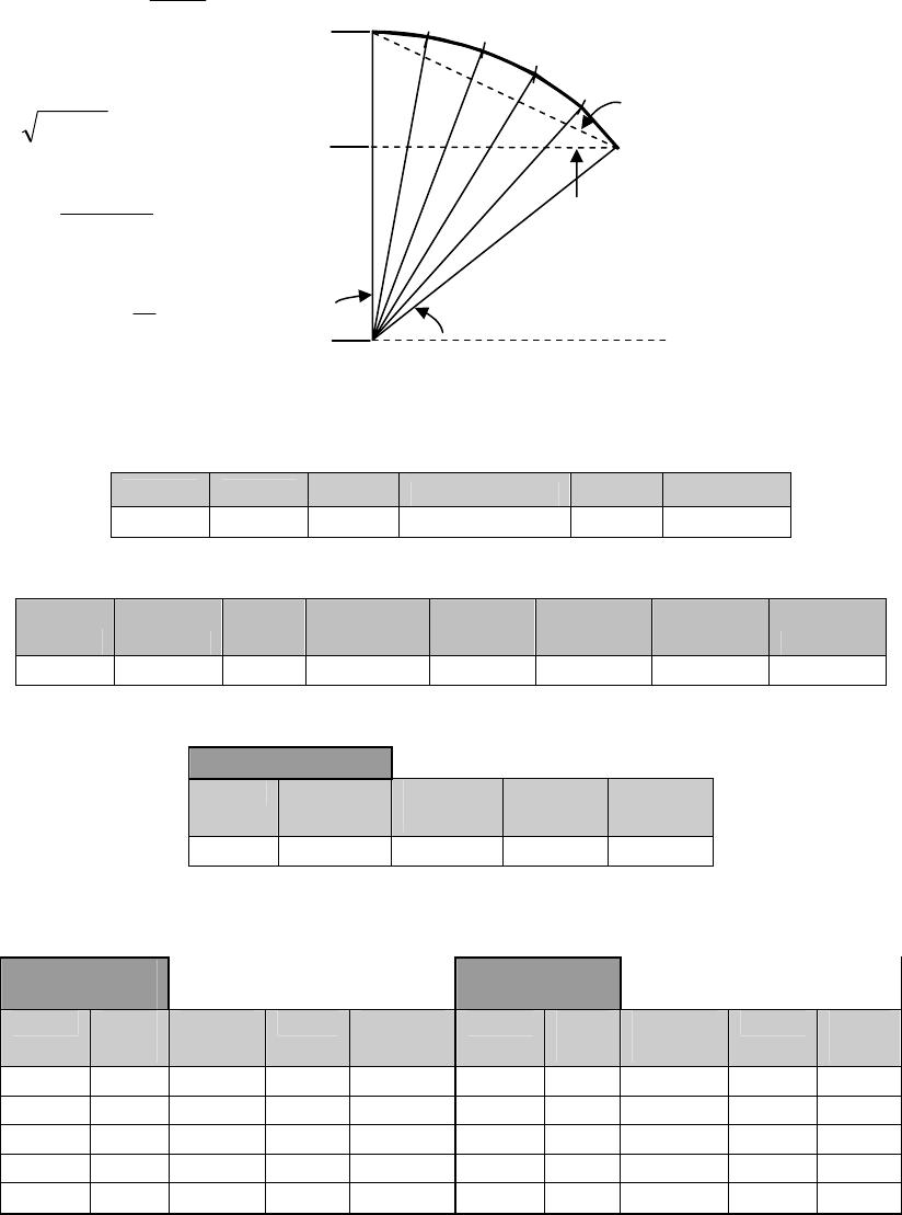
The numbering of the regions is contained in the following sketch

Before performing the characteristic calculations, various geometric calculations must be

made. Development of the relations is straightforward. The symbols are labeled in the

sketch below.

851177.1M =

∞

cm 407417.3t

=

cm 100R

=

M∞ = 1.851177

2

Region 1

4

3

6

5

7

8

9

10

11

Type I

Type II

this material may be reproduced, in any form or by any means, without permission in writing from the publisher.

333

⎟

⎠

⎞

⎜

⎝

⎛−

−= −

R

tR

cosAOT 1

()

AOTsinRl −−=

22 ltc +=

()

n

AOTR

L−=∆

⎟

⎠

⎞

⎜

⎝

⎛

=−

R

t

tanAOA 1

Input data and the initial calculations for the problem are contained in the following:

γ α1 n M∞ = M1 R t

1.4 0 5 1.851177 100 3.407417

ν1 p1/po AOT ∆α = α4 /n l c ∆L AOA

22.1970 0.16090 -15 -3.0000 25.8819 26.1052 5.2360 7.5000

FREESTREAM

Region α

deg

ν

deg

M p/po

1 0.0 22.1970 1.8512 0.1609

Following the region-to-region procedure (see the solution to Problem 18)

UPPER

SURFACE

LOWER

SURFACE

Region α

deg

ν

deg

M p/po

Region α

deg

ν

deg

M p/po

2 -3.0 25.1970 1.9573 0.1366 7 -3.0 19.1970 1.7474 0.1886

3 -6.0 28.1970 2.0665 0.1152 8 -6.0 16.1970 1.6452 0.2200

4 -9.0 31.1970 2.1794 0.0966 9 -9.0 13.1970 1.5438 0.2556

5 -12.0 34.1970 2.2966 0.0804 10 -12.0 10.1970 1.4417 0.2962

6 -15.0 37.1970 2.4187 0.0664 11 -15.0 7.1970 1.3371 0.3431

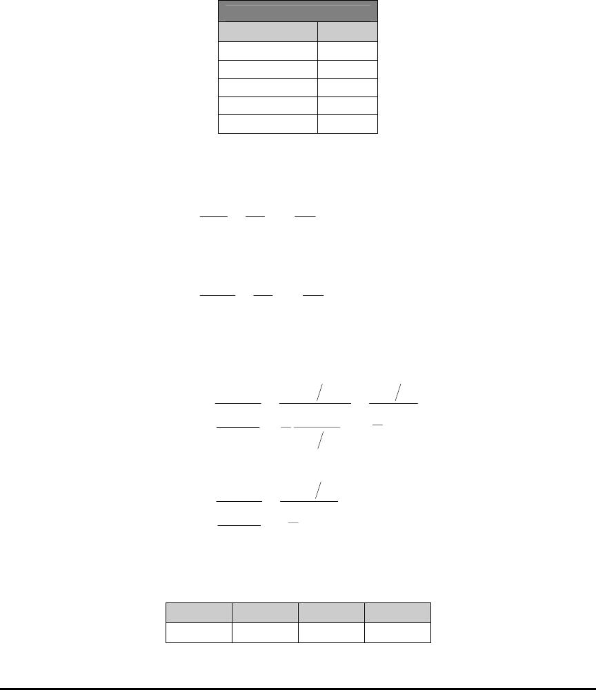
Next the pressure difference across the airfoil, i.e., the pressure on the upper surface is

subtracted from the pressure on the lower surface, is determined

c

an

g

le of turn

(

AOT

)

R

∆

L

l

t

∆

L

∆

L

∆

L

∆

L

an

g

le of attack

(

AOA

)

R – t

this material may be reproduced, in any form or by any means, without permission in writing from the publisher.

334

(plower – pupper)

Segment ∆p/po

1 (R7 – R2) 0.05201

2 (R8 – R3) 0.10474

3 (R9 – R4) 0.15900

4 (R10 – R5) 0.21579

5 (R11 – R6) 0.27662

The lift and drag forces are computed from

i

5

1i i

o1

o

1

i

5

1i i

o1

o

1

sinL

p

Drag

cosL

p

Lift

α∆

⎟

⎠

⎞

⎜

⎝

⎛∆

=

α∆

⎟

⎠

⎞

⎜

⎝

⎛∆

=

∑

=

The lift and drag coefficients are computed from

cM

2

pDrag

2

cV

Drag

C

cM

2

pLift

c

p

V

2

pLift

2

cV

Lift

C

2

1

2

11

D

2

1

11

2

1

2

11

L

γ

=

ρ

=

γ

=

ργ

γ

=

ρ

=

The results of the calculations are

Lift/p∞ Drag/p∞ CL CD

0.25754 0.05044 0.41126 0.08055

Problem 21. –A converging-diverging nozzle discharges a uniform supersonic flow at

Mach 2.2 and static pressure of 101 kPa two dimensionally into a back pressure region of

69.28701 kPa. Use the Region-to-Region method to determine the flow just downstream

of the nozzle exit for the same configuration as employed in Example 14.4. Assume

γ = 1.4.

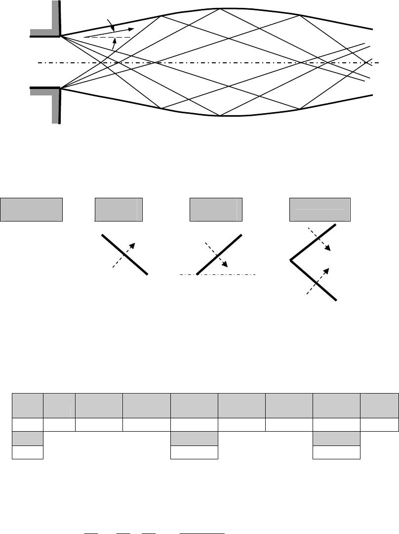
Because this problem follows that of Example 14.4 for the same configuration, the figure

of that example is repeated below

this material may be reproduced, in any form or by any means, without permission in writing from the publisher.

335

The calculation procedure for the region-to-region method is given as

α4 calc

x’g Type

I

x’g Type

II Combined

∆ν = −∆α

ν4 − ν1 = α4 − α1

α4 = α1 + ν4 − ν1

∆α = α4 /n

∆ν = ∆α

n = no of divisions ∆ν = ∆α ∆ν = −∆α

ν2 − ν1 = α2 − α1 ν5 − ν2 = −(α5 − α2) ν6 = [(ν5 − α5) + (ν3 + α3)]/2

ν2 = ν1 + ∆α ν5 = ν2 + α2 α

6 = ν6 − (ν5 − α5)

The initial and computed data for this problem follows

γ α1 pe = p1 pb = p4 Me = M1 pe/po p4/po M4

∆α =

α4 /n

1.4 0 101 69.28701 2.2 0.09352 0.06416 2.4410 2.0000

n ν1

ν4

3 31.7325 37.7325

Because Region 4 is a uniform flow region bordering the free surface: p4 = 69.28701 kPa.

For isentropic flow at M1 = 2.2 and γ = 1.4,

()

06416.009352.0

101

28701.69

p

o

1

4

o

4=

⎟

⎠

⎞

⎜

⎝

⎛

=

⎟

⎠

⎞

⎜

⎝

⎛

⎟

⎠

⎞

⎜

⎝

⎛

=

So using the isentropic flow solver for this pressure ratio we find 4410.2M4

=

as shown

above.

Me

p

b

14

10

9

15

19 21

20

3

2

1

5

4

7

6

812

11

13

16

17 18

p

e

α4

αe

1

2

5

3

6

α

5 = 0

this material may be reproduced, in any form or by any means, without permission in writing from the publisher.

336

At this Mach number, from the Prandtl-Meyer Spreadsheet Solver (PMSS):

ν4 = 37.7325° and µ4 = sin−1(1/ M4) = 24.1836°. Also at M1 = 2.2, the PMSS gives ν1 =

31.7325° and µ1 = sin−1(1/ M1) = 27.0357°. Hence,

o

0000.67325.317325.370.0

1414 =−+=ν−ν+α=α

As seen in Figure 14.16, the expansion fan has been divided into 3 equal pieces so that

oo 0.4 ,0.2

3

0.6

32 =α==α

The results of the calculations are listed below

Region α

deg

ν

deg

M µ

deg

α + µ

deg

α − µ

deg

1 0.0 31.7325 2.2 27.0357 27.0357 -27.0357

2 2.0000 33.7325 2.2781 26.0373 28.0373 -24.0373

3 4.0000 35.7325 2.3584 25.0883 29.0883 -21.0883

4 6.0000 37.7325 2.4410 24.1836 30.1836 -18.1836

5 0.0 35.7325 2.3584 25.0883 25.0883 -25.0883

6 2.0000 37.7325 2.4410 24.1836 26.1836 -22.1836

7 4.0000 39.7325 2.5262 23.3189 27.3189 -19.3189

8 2.0000 37.7325 2.4410 24.1836 26.1836 -22.1836

9 0.0 39.7325 2.5262 23.3189 23.3189 -23.3189

10 2.0000 41.7325 2.6142 22.4905 24.4905 -20.4905

11 0.0000 39.7325 2.5262 23.3189 23.3189 -23.3189

12 -2.0000 37.7325 2.4410 24.1836 22.1836 -26.1836

13 0.0 43.7325 2.7051 21.6951 21.6951 -21.6951

14 -2.0000 41.7325 2.6142 22.4905 20.4905 -24.4905

15 -4.0000 39.7325 2.5262 23.3189 19.3189 -27.3189

16 -6.0000 37.7325 2.4410 24.1836 18.1836 -30.1836

17 0.0 39.7325 2.5262 23.3189 23.3189 -23.3189

18 -2.0000 37.7325 2.4410 24.1836 22.1836 -26.1836

19 -4.0000 35.7325 2.3584 25.0883 21.0883 -29.0883

20 0.0 39.7325 2.5262 23.3189 23.3189 -23.3189

21 -2.0000 37.7325 2.4410 24.1836 22.1836 -26.1836

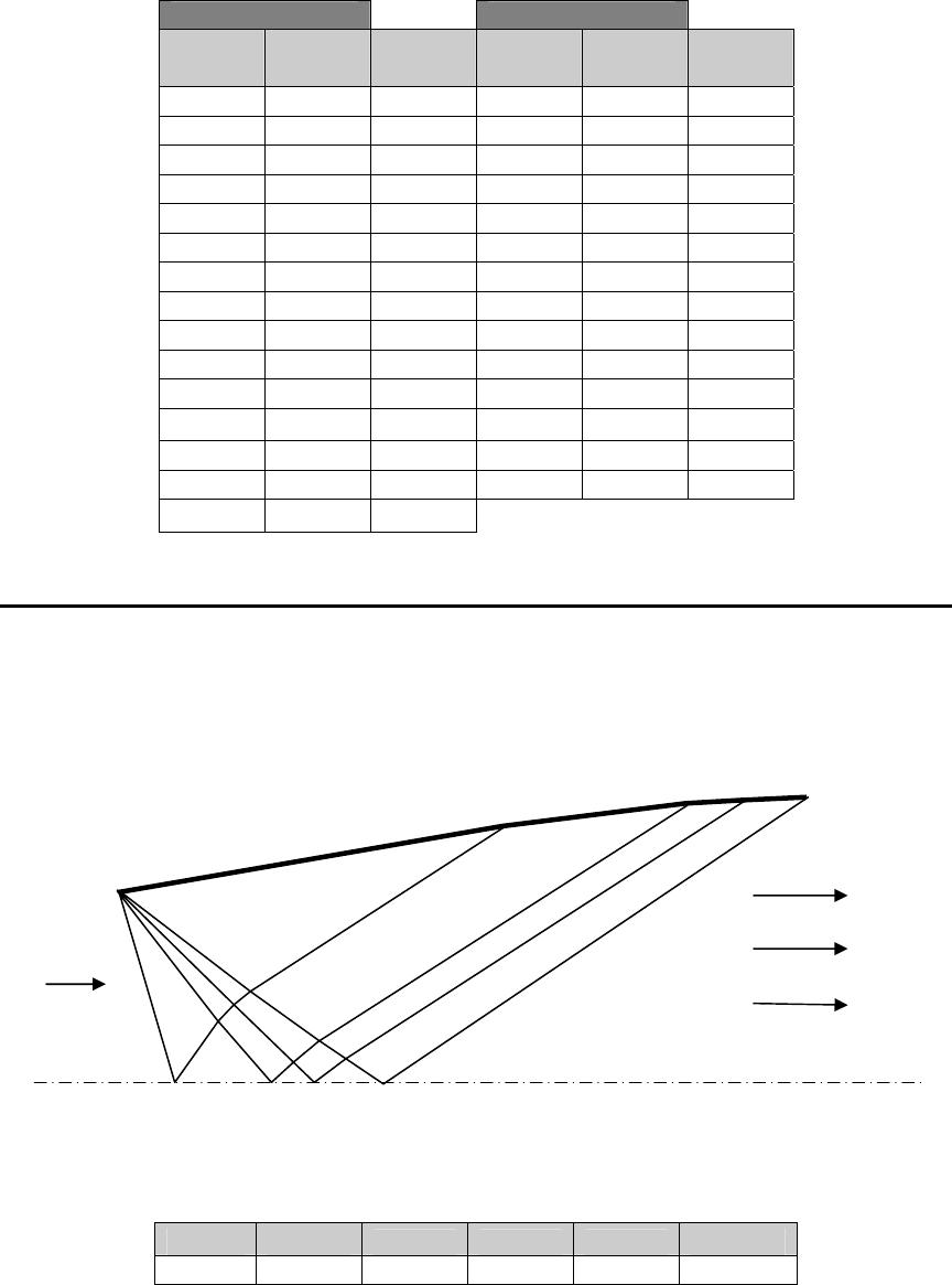
The averaged angles of inclination and the slopes of the characteristics are

this material may be reproduced, in any form or by any means, without permission in writing from the publisher.

337

Type I: α − µ Type II: α + µ

Regions Angle

deg

slopeI Regions Angle

deg

slopeII

1 – 2 -25.5365 -0.4778 2 – 5 26.5628 0.5000

2 – 3 -22.5628 -0.4155 3 – 6 27.6359 0.5236

3 – 4 -19.6359 -0.3568 4 – 7 28.7513 0.5486

5 – 6 -23.6359 -0.4376 6 – 9 24.7513 0.4610

6 – 7 -20.7513 -0.3789 7 – 10 25.9047 0.4857

7 – 8 -20.7513 -0.3789 8 – 11 24.7513 0.4610

9 – 10 -21.9047 -0.4021 10 – 13 23.0928 0.4264

10 – 11 -21.9047 -0.4021 11 – 14 21.9047 0.4021

11 – 12 -24.7513 -0.4610 12 – 15 20.7513 0.3789

13 – 14 -23.9394 -0.4440 14 – 17 21.9047 0.4021

14 – 15 -23.0928 -0.4264 15 – 18 20.7513 0.3789

15 – 16 -25.9047 -0.4857 16 – 19 19.6359 0.3568

17 – 18 -28.7513 -0.5486 18 – 20 22.7513 0.4194

18 – 19 -26.7513 -0.5041 19 – 21 21.6359 0.3967

20 – 21 -24.7513 -0.4610

Problem 22. –Repeat Example 14.5 using the region-to-region method. Compare the

results.

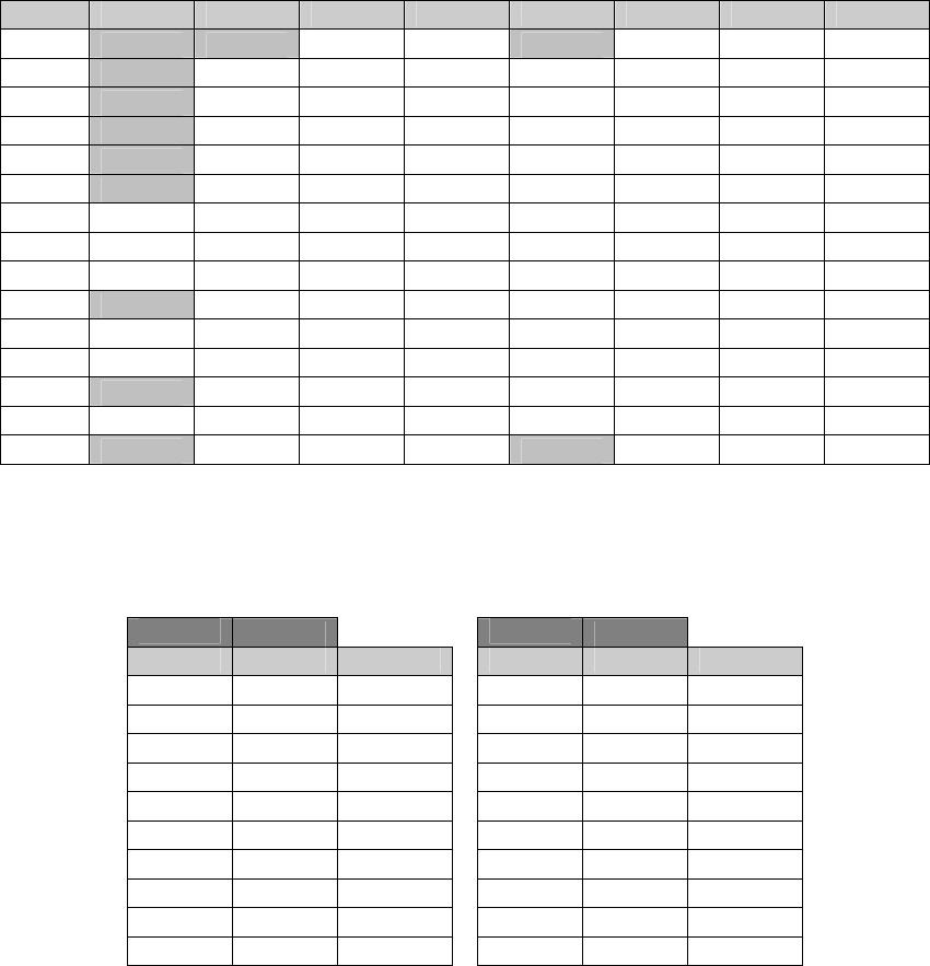
The numbering and layout of the regions is contained in the following sketch

Input and the maximum turning angle are contained in the following table

γ α1 M1 M15 divisions αw,max,MLN

1.2 0 1 1.8 4 12.151243

Using this information and the region-to-region methodology explained in Problem 18

we can determine the values in the table which follows

1 2 3 4

5

6 7 8

9

10 11

12 14

13

15

M15

M1

this material may be reproduced, in any form or by any means, without permission in writing from the publisher.

338

Region α ν I = ν+α II = ν−α M µ α + µ α − µ

1 0.0000 0.0000 0.0000 0.0000 1.0000 90.0000 90.0000 -90.0000

2 3.0378 3.0378 6.0756 0.0000 1.1659 59.0617 62.0995 -56.0239

3 6.0756 6.0756 12.1512 0.0000 1.2727 51.7871 57.8627 -45.7115

4 9.1134 9.1134 18.2269 0.0000 1.3682 46.9605 56.0740 -37.8471

5 12.1512 12.1512 24.3025 0.0000 1.4583 43.2931 55.4444 -31.1419

6 0.0000 6.0756 6.0756 6.0756 1.2727 51.7871 51.7871 -51.7871

7 3.0378 9.1134 12.1512 6.0756 1.3682 46.9605 49.9984 -43.9227

8 6.0756 12.1512 18.2269 6.0756 1.4583 43.2931 49.3687 -37.2175

9 9.1134 15.1891 24.3025 6.0756 1.5454 40.3208 49.4342 -31.2074

10 0.0000 12.1512 12.1512 12.1512 1.4583 43.2931 43.2931 -43.2931

11 3.0378 15.1891 18.2269 12.1512 1.5454 40.3208 43.3586 -37.2830

12 6.0756 18.2269 24.3025 12.1512 1.6309 37.8175 43.8931 -31.7418

13 0.0000 18.2269 18.2269 18.2269 1.6309 37.8175 37.8175 -37.8175

14 3.0378 21.2647 24.3025 18.2269 1.7156 35.6540 38.6918 -32.6162

15 0.0000 24.3025 24.3025 24.3025 1.8000 33.7490 33.7490 -33.7490

The angles of inclinations of the characteristics can be used to determine the x,y locations

of characteristics. These are determined by averaging the characteristic angles, α ± µ , of

adjoining regions.

Type I

Type II

Region Region Inclinat’n Region Region Inclinat’n

1 2 -73.0120 2 6 56.9433

2 3 -50.8677 3 7 53.9305

3 4 -41.7793 4 8 52.7214

4 5 -34.4945 5 9 52.4393

6 7 -47.8549 7 10 46.6457

7 8 -40.5701 8 11 46.3637

8 9 -34.2124 9 12 46.6637

10 11 -40.2881 11 13 40.5880

11 12 -34.5124 12 14 41.2924

13 14 -35.2168 14 15 36.2204

this material may be reproduced, in any form or by any means, without permission in writing from the publisher.