978-0131206687 Chapter 13

272

Chapter Thirteen

L

LI

IN

NE

EA

AR

RI

IZ

ZE

ED

D

F

FL

LO

OW

WS

S

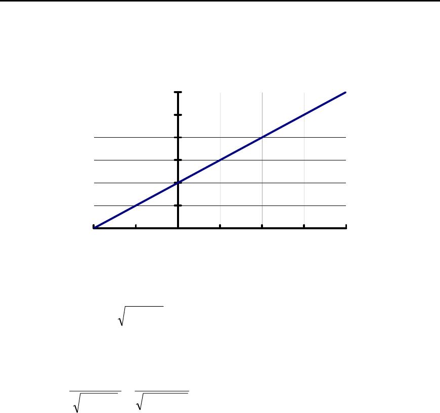
Problem 1. – The lift coefficient versus angle of attack for an airfoil, as measured in a

low-speed wind tunnel, is given in Figure P13.1. Sketch this curve for the same airfoil at

a Mach number of 0.45.

0.0

0.2

0.4

0.6

0.8

1.0

1.2

–4–202468

Figure P13.1

From the Prandtl Glauert similarity rule, we can write

2

L0ML M1CC ∞=

∞−=

Therefore,

0ML

2

0ML

2

0ML

LC1198.1

45.01

C

M1

C

C=

∞

=

∞

=

∞=

−

=

−

=

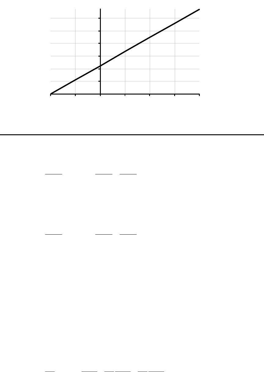
Using this result and the values of 0ML

C=

∞ from Figure P13.1 we can sketch the lift

coefficient versus angle of attack for the same airfoil at a Mach number of 0.45

CL

α (degrees)

this material may be reproduced, in any form or by any means, without permission in writing from the publisher.

273

0

0.2

0.4

0.6

0.8

1

1.2

-4 -2 0 2 4 6 8

α (degrees)

C

L

Problem 2. – Using the potential equation

()

0

zy

M1

x2

p

2

p

2

p

2

=

∂

φ∂

+

∂

φ∂

+−

∂

φ∂

∞

develop the Goethert similarity rules for three-dimensional potential subsonic flow.

The equation

()

0

zy

M1

x2

p

2

p

2

p

2

=

∂

φ∂

+

∂

φ∂

+−

∂

φ∂

∞

is for small-perturbation, linearized compressible three-dimensional flow. We transform

this flow to an incompressible flow. Let

xkx 1i =

yky 2i =

zkz 3i =

φ=φ 4i k

∞∞ =UkU 5i

and substitute into the potential equation:

()

0

z

k

y

k

x

M1

k

2

i

2

4

2

3

2

i

2

4

2

i

2

4

2

1=

∂

φ∂

+

∂

φ∂

+

∂

φ∂

−∞

this material may be reproduced, in any form or by any means, without permission in writing from the publisher.

274

Multiplying this equation with 324 kkk we obtain:

()

0

z

k

y

k

x

M1

kk

k

2

i

2

3

2

i

2

3

2

i

2

32

2

1=

∂

φ∂

+

∂

φ∂

+

∂

φ∂

−∞

In order to transform the potential equation for compressible flow into Laplace’s

equation, it follows that

2

32

1

M1

1

kk

k

∞

−

=

1

k

3

2=

The boundary conditions for the three-dimensional compressible flow are:

∞

=

⎟

⎠

⎞

⎜

⎝

⎛

U

v

dx

dy p

b

∞

=

⎟

⎠

⎞

⎜

⎝

⎛

U

w

dx

dz p

b

where

y

vp

p∂

φ∂

=

z

wp

p∂

φ∂

=

Transforming the boundary conditions to the incompressible flow, we have:

4

52

i

ip

i

b

i

2

1

k

kk

yU

1

dx

dy

k

∂

φ

∂

=

⎟

⎠

⎞

⎜

⎝

⎛

∞

4

53

i

ip

i

b

i

3

1

k

kk

zU

1

dx

dz

k

∂

φ

∂

=

⎟

⎠

⎞

⎜

⎝

⎛

∞

To satisfy the boundary conditions for the incompressible flow, it is necessary that

4

52

2

1

k

kk

k

k=

4

53

3

1

k

kk

k

k=

this material may be reproduced, in any form or by any means, without permission in writing from the publisher.

275

For the incompressible flow, the Bernoulli’s equation is:

(

)

[

]

2

pi

2

pi

2

piii

2

i

iwvuU

2

1

pU

2

1

p+++ρ+=ρ+ ∞

∞

or

⎥

⎦

⎤

⎢

⎣

⎡

⎟

⎠

⎞

⎜

⎝

⎛

−

⎟

⎠

⎞

⎜

⎝

⎛

−

⎟

⎠

⎞

⎜

⎝

⎛

−−ρ=−

∞∞∞∞

∞

2

i

pi

2

i

pi

2

i

pi

i

pi

2

i

ii U

w

U

v

U

u

U

u2

U

2

1

pp

Introducing this equation into

2

i

ii

i

p

U

2

1

pp

C

∞

ρ

−

=

and dropping the smaller terms, we receive

i

pi

i

pU

u2

C

∞

−=

For the compressible flow we have

pi

4

51

4

51

i

pi

p

pC

k

kk

k

kk

U

x

2

U

x

2

U

u2

C=

∂

φ

∂

−=

∂

φ∂

−=−=

∞∞∞

or

pi

2

pC

M1

1

C

∞

−

=

Problem 3. – Tests run at 3.0M =

∞show that the lift coefficient versus angle of attack

for an airfoil is given by

(

)

11.0CL

+

α

=

with

α

in degrees. Using the appropriate

similarity laws, derive an expression for L

C versus

α

for this airfoil at 5.0M =

∞.

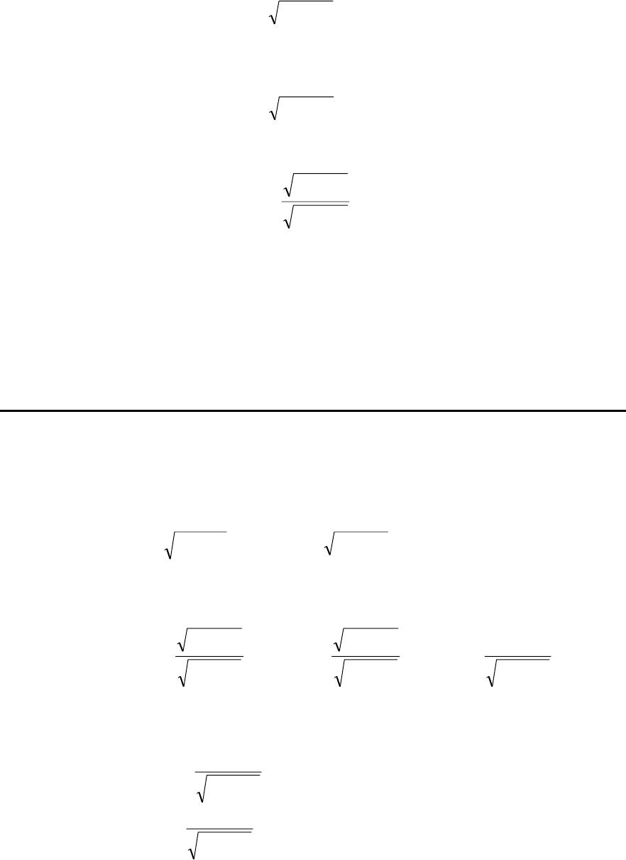
Using the Prandtl Glauert similarity rule

2

L0ML M1CC ∞=

∞−=

we obtain

this material may be reproduced, in any form or by any means, without permission in writing from the publisher.

276

2

3.0ML0ML 3.01CC −= =

∞

=

∞

and

2

5.0ML0ML 5.01CC −= =

∞

=

∞

Therefore,

10.1C

5.01

3.01

CC 3.0ML

2

3.0ML5.0ML =

∞

=

∞

=

∞=

−

=

But

()

11.0C 3.0ML

+

α

=

∞

and the expression for L

C versus

α

at 5.0M

=

∞ is

()

(

)

111.010.111.0C 5.0ML

+

α

=

+α=

=

∞

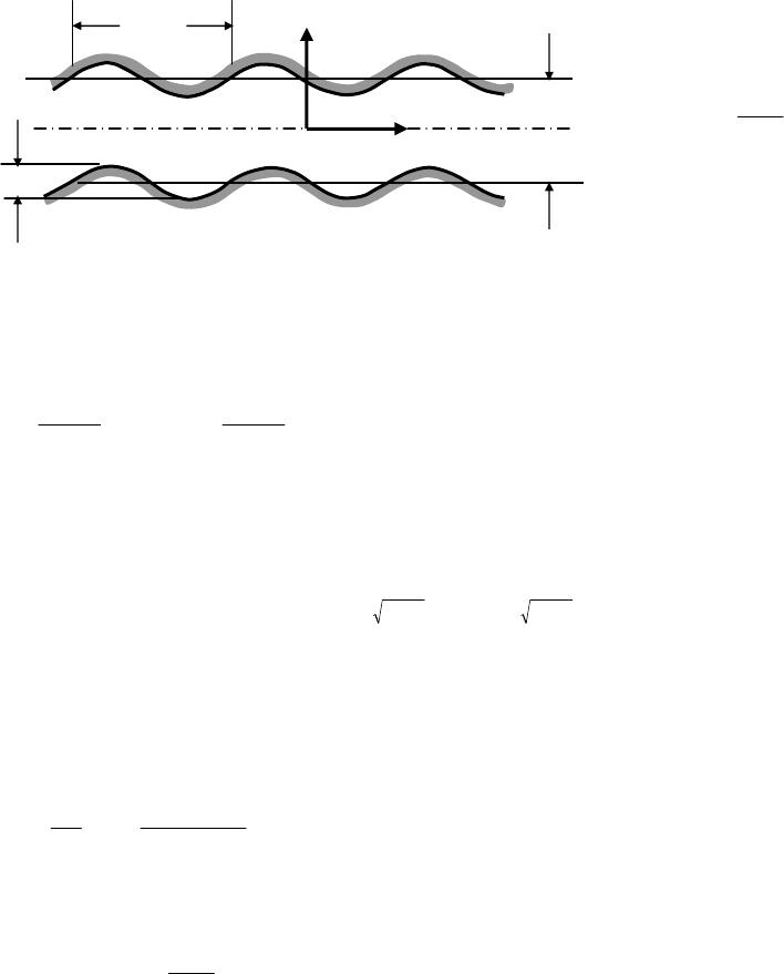
Problem 4. – For the airfoil of Problem 3, plot CL versus M∞ from M∞ = 0 to M∞ = 0.60 at

angles of attack of 0○, 2○ and 4○.

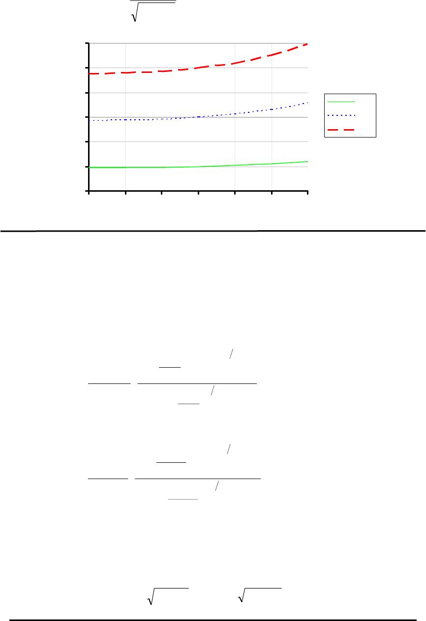
From the Prandtl Glauert similarity rule we have

2

3.0ML

2

L0ML 3.01CM1CC −=−= =

∞

∞=

∞

or

() ()

22

2

3.0MLL

M1

1

095394.0

M1

3.01

11.0

M1

3.01

CC

∞∞∞

=

∞−

+α

=

−

+α=

−

=

Therefore,

2

0L M1

1

095394.0C

∞

=α −

=

o

2

2L M1

1

28618.0C

∞

=α −

=

o

this material may be reproduced, in any form or by any means, without permission in writing from the publisher.

277

2

4L M1

1

47697.0C

∞

=α −

=

o

0

0.1

0.2

0.3

0.4

0.5

0.6

0 0.1 0.2 0.3 0.4 0.5 0.6

M

∞

CL

α=0

α=2

α=4

Problem 5. – During the testing of a two-dimensional, streamlined shape, it is found that

sonic flow first occurs on the surface for 70.0M

=

∞. Calculate the pressure coefficient at

this point and also the minimum pressure coefficient for this shape in incompressible

flow.

The pressure coefficient in the point in which the sonic flow occurs is

(

)

()

779.01

2

14.1

1

7.0

2

14.1

1

7.04.1

2

1

2

1

M

2

1

M

2

C

14.14.1

2

1

2

crit

2

crit

1Mp

−=

⎥

⎦

⎤

⎢

⎣

⎡

−

⎟

⎠

⎞

⎜

⎝

⎛−

+

⎟

⎠

⎞

⎜

⎝

⎛−

+

=

⎥

⎦

⎤

⎢

⎣

⎡

−

⎟

⎠

⎞

⎜

⎝

⎛−γ

+

⎟

⎠

⎞

⎜

⎝

⎛−γ

+

γ

=

−

−γγ

∞

=

The minimum pressure coefficient in incompressible flow is calculated from the Prandtl

Glauert rule

556.07.01779.0M1CC 22

Mp0Mp −=−−=−= ∞= ∞∞

this material may be reproduced, in any form or by any means, without permission in writing from the publisher.

278

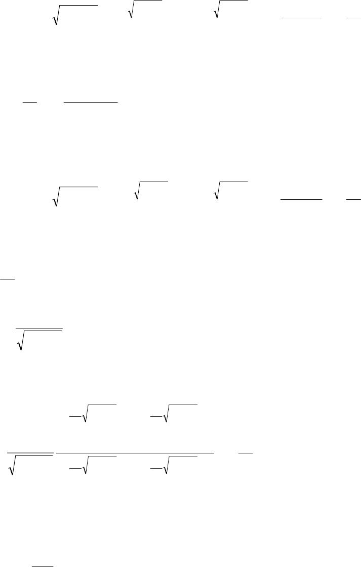
Problem 6. – Two-dimensional subsonic linearized potential flow takes place between

two wavy walls as shown Figure P13.6. Solve for p

φ

and determine the pressure

distribution along the centerline.

Figure P13.6

The potential equation for two-dimensional compressible flow is

()

0

y

M1

x2

p

2

p

2

=

∂

φ∂

+−

∂

φ∂

∞

For subsonic flow, the solution of this equation can be obtained using the method of

separation of variables

()

⎟

⎠

⎞

⎜

⎝

⎛++=φ ∞∞ −−− kyM1

4

kyM1

321p

22 ececkxsinckxcosc

The constants c1, c2, c3, c4 can be determined from the boundary conditions. For dy

=

,

the boundary condition is

()

∞

=

⎟

⎠

⎞

⎜

⎝

⎛

U

d,xv

dx

dy bp

b

where

()

y

d,xv p

bp ∂

φ∂

=

Introducing the relationships for b

y and for p

φ

into the boundary condition we receive a

condition between the constants c1, c2, c3, c4

d

x2

sinAy ±

⎟

⎠

⎞

⎜

⎝

⎛

λ

π

=

d

λ

2A

x

y

A << d

this material may be reproduced, in any form or by any means, without permission in writing from the publisher.

279

()

⎟

⎠

⎞

⎜

⎝

⎛

λ

π

λ

π

=

⎟

⎠

⎞

⎜

⎝

⎛−−+ ∞

∞

−−

∞

−

∞x

2

cos

AU2

ececkM1kxsinckxcosc kd

2

M1

4

kd

2

M1

3

2

21

Similarly, for dy−= we have

()

∞

−

=

⎟

⎠

⎞

⎜

⎝

⎛

U

d,xv

dx

dy bp

b

or

()

⎟

⎠

⎞

⎜

⎝

⎛

λ

π

λ

π

=

⎟

⎠

⎞

⎜

⎝

⎛−−+ ∞

∞

−

∞

−−

∞x

2

cos

AU2

ececkM1kxsinckxcosc kd

2

M1

4

kd

2

M1

3

2

21

From the two relations between the constants c1, c2, c3, c4 we obtain

λ

π

=2

k

0c2=

2

31

M1

AU

cc

∞

−

=

With these relations, the potential function p

φ

is

⎟

⎠

⎞

⎜

⎝

⎛

λ

π

⎟

⎠

⎞

⎜

⎝

⎛

+

⎟

⎠

⎞

⎜

⎝

⎛

−

=φ

∞

−

λ

π

−

∞

−

λ

π

∞

−

λ

π

−

∞

−

λ

π

∞

∞x

2

cos

ee

M1

AU

d

2

M1

2

d

2

M1

2

y

2

M1

2

y

2

M1

2

p

Along the centerline we have

0

x

u

0y

p

0yp =

⎟

⎠

⎞

⎜

⎝

⎛

∂

φ∂

=

which implies

this material may be reproduced, in any form or by any means, without permission in writing from the publisher.

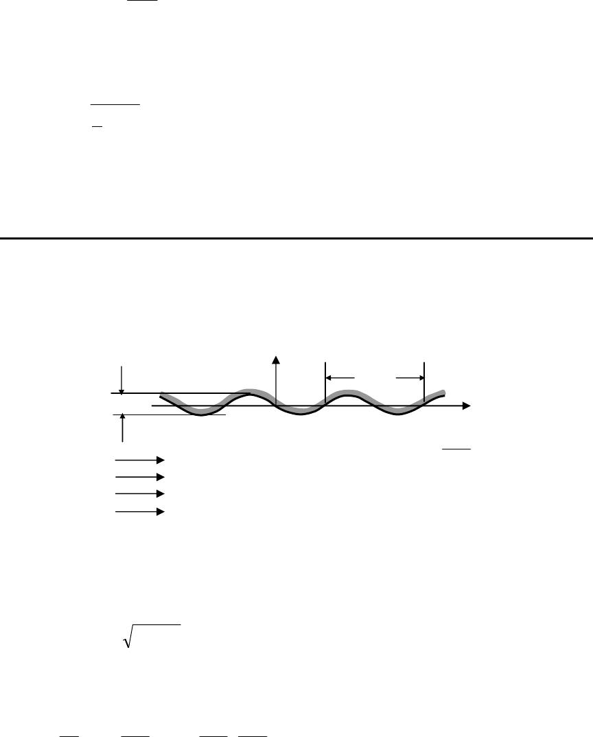
280

0

U

u2

Cp

0yp =−=

∞

=

Because

2

p

U

2

1

pp

C

∞

ρ

−

=

we obtain that along the centerline the pressure is constant

∞

=pp

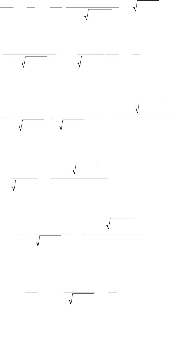
Problem 7. – Consider two-dimensional, supersonic, linearized flow under a wavy wall,

as shown in Figure P13.7. Solve for the velocity potential of the flow and pressure

coefficient along the wall. Derive an expression for the lift and drag per wave length.

Figure P13.7

The general solution of the linearized potential equation two-dimensional, supersonic

flow under a wall is

(

)

y1Mxf 2

p−+=φ ∞

The boundary condition is

0y

p

0y

byU

1

U

v

dx

dy

=

∞

=

∞⎟

⎟

⎠

⎞

⎜

⎝

⎛

∂

φ∂

=

⎟

⎠

⎞

⎜

⎝

⎛

=

⎟

⎠

⎞

⎜

⎝

⎛

For the wavy wall, this boundary condition becomes

M∞

p∞

λ

2A

y

x

⎟

⎠

⎞

⎜

⎝

⎛

λ

π

=x2

sinAyb

this material may be reproduced, in any form or by any means, without permission in writing from the publisher.

281

1M

y1Mxd

df

U

1

x

2

cos

A2 2

0y

2

−

⎥

⎦

⎤

⎢

⎣

⎡

⎟

⎠

⎞

⎜

⎝

⎛−+

=

⎟

⎠

⎞

⎜

⎝

⎛

λ

π

λ

π∞

=

∞

⎟

⎠

⎞

⎜

⎝

⎛

λ

π

λ

π

−

=

⎥

⎦

⎤

⎢

⎣

⎡

⎟

⎠

⎞

⎜

⎝

⎛−+ ∞

∞

=

∞

x

2

cos

A2

1M

U

y1Mxd

df

2

0y

2

or, any y,

⎟

⎠

⎞

⎜

⎝

⎛

λ

⎟

⎠

⎞

⎜

⎝

⎛−+π

λ

π

−

=

⎟

⎠

⎞

⎜

⎝

⎛−+

∞

y1Mx2

cos

A2

1M

U

y1Mxd

df

2

Integrating, we obtain

p

2

2constant

y1Mx2

sin

1M

AU

fφ=+

⎟

⎠

⎞

⎜

⎝

⎛

λ

⎟

⎠

⎞

⎜

⎝

⎛−+π

−

=∞

∞

The perturbation velocity p

u is

⎟

⎠

⎞

⎜

⎝

⎛

λ

⎟

⎠

⎞

⎜

⎝

⎛−+π

λ

π

−

=

∂

φ∂

=∞

∞

∞y1Mx2

cos

2

1M

AU

x

u

2

p

With p

u we can compute the pressure coefficient p

C along the wall

⎟

⎠

⎞

⎜

⎝

⎛

λ

π

−λ

π

−=

⎟

⎠

⎞

⎜

⎝

⎛−=

∞

=

∞

x

2

cos

1M

A4

U

u2

C2

0y

p

The differential lift dL is given by

dxpdxMp

2

1

CdL 2

p∞∞∞ +γ=

this material may be reproduced, in any form or by any means, without permission in writing from the publisher.

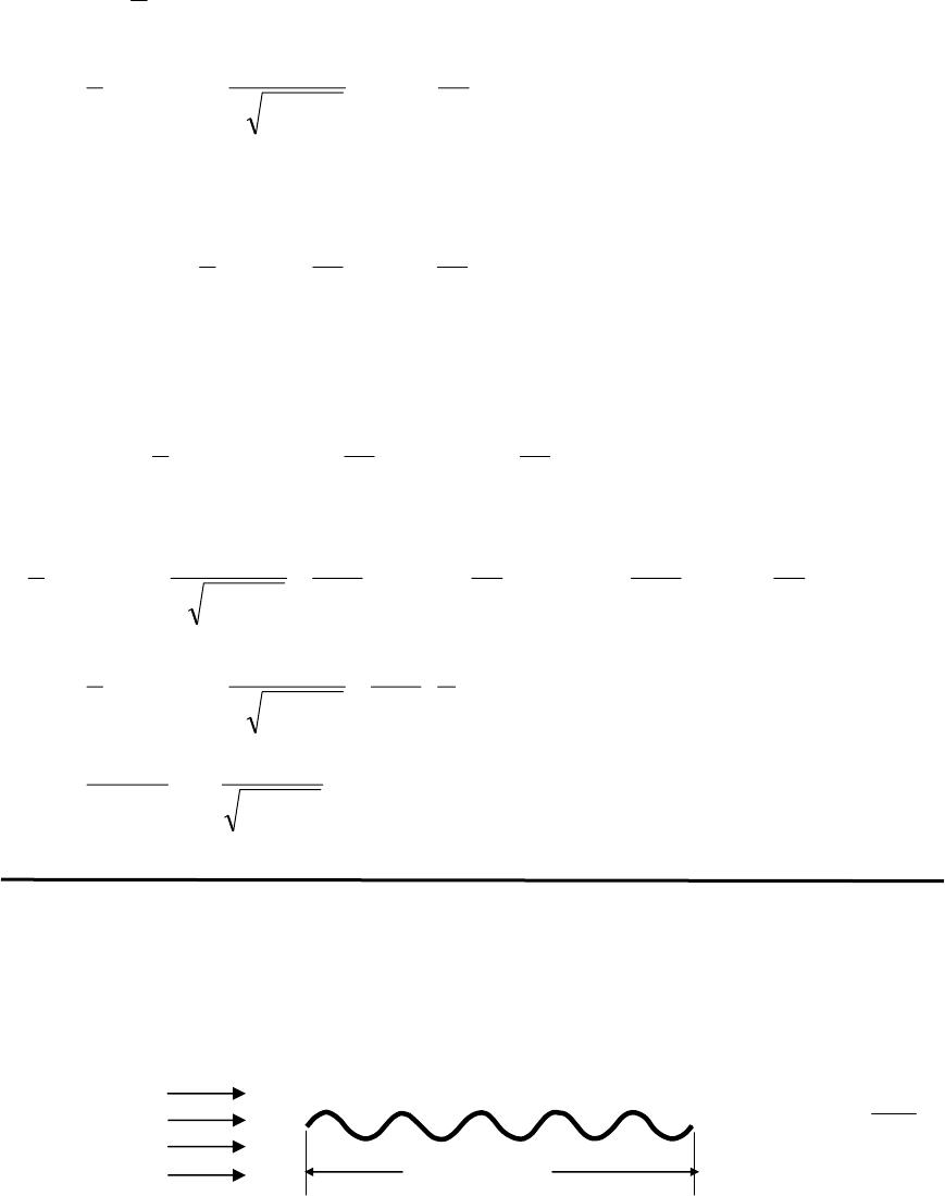
282

where lift is defined to be positive upward.

Integrating from 0 to λ, we obtain the lift force per wave length

=+γ= ∫∫ λ∞

λ

∞∞ dxpdxCMp

2

1

L00 p

2

λ=+

⎟

⎠

⎞

⎜

⎝

⎛

λ

π

⎟

⎠

⎞

⎜

⎝

⎛

−λ

π

−γ ∞

λ

∞

λ

∞

∞∞ ∫∫ pdxpdxx

2

cos

1M

A4

Mp

2

1

00

2

The differential drag is

dx

dy

pdx

dx

dy

Mp

2

1

CdD 2

p∞∞∞ −γ−=

where drag is positive in the flow direction. Integrating from 0 to λ, we have the drag per

wave length

=

⎟

⎠

⎞

⎜

⎝

⎛

−

⎟

⎠

⎞

⎜

⎝

⎛

γ−= ∫∫ λ∞

λ

∞∞ dx

dx

dy

pdx

dx

dy

CMp

2

1

D00 p

2

=

⎟

⎠

⎞

⎜

⎝

⎛

λ

π

⎟

⎠

⎞

⎜

⎝

⎛

λ

π

−

⎟

⎠

⎞

⎜

⎝

⎛

λ

π

⎟

⎠

⎞

⎜

⎝

⎛

λ

π

⎟

⎠

⎞

⎜

⎝

⎛

−λ

π

−γ− ∫∫ λ

∞

λ

∞

∞∞ dxx

2

cos

A2

pdxx

2

cos

A2

1M

A4

Mp

2

1

00

2

=

λ

⎟

⎠

⎞

⎜

⎝

⎛

λ

π

⎟

⎠

⎞

⎜

⎝

⎛

−λ

π

−γ

∞

∞∞ 2

A2

1M

A4

Mp

2

1

2

1M

M

p

A2

2

22

−

γ

λ

π

∞

Problem 8. – A wing has the shape of a sine wave, as shown in Figure P13.8. Compute

the lift and drag for supersonic flow. Assume linearized, two-dimensional flow above and

below the foil.

Figure P13.8

M∞

p∞ Chord

= 5λ

⎟

⎠

⎞

⎜

⎝

⎛

λ

π

=x2

sinAyb

this material may be reproduced, in any form or by any means, without permission in writing from the publisher.

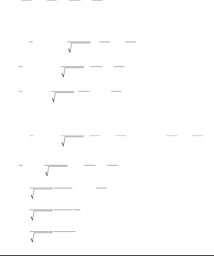
283

For a wing with a shape of a sine wave we have

⎟

⎠

⎞

⎜

⎝

⎛

λ

π

λ

π

=

⎟

⎠

⎞

⎜

⎝

⎛

=

⎟

⎠

⎞

⎜

⎝

⎛x2

cos

A2

dx

dy

dx

dy

u

b

L

b

Introducing these relations in the expression of the lift for an airfoil, we have

=

⎪

⎭

⎪

⎬

⎫

⎪

⎩

⎪

⎨

⎧⎟

⎠

⎞

⎜

⎝

⎛

+

⎟

⎠

⎞

⎜

⎝

⎛

⎟

⎠

⎞

⎜

⎝

⎛

−

−γ= ∫

∞

∞∞ dx

dx

dy

dx

dy

1M

2

Mp

2

1

L

u

b

L

b

c

02

2

=

⎟

⎠

⎞

⎜

⎝

⎛

λ

π

λ

π

⎟

⎠

⎞

⎜

⎝

⎛

−

−γ ∫λ

∞

∞∞ dx

x2

cos

A2

2

1M

2

Mp

2

15

02

2

0dx

x2

cos

A4

1M

2

Mp

2

15

0

2

2=

⎟

⎠

⎞

⎜

⎝

⎛

λ

π

λ

π

⎟

⎠

⎞

⎜

⎝

⎛

−

−γ ∫λ

∞

∞∞

For the drag, in the same manner we have

=

⎥

⎦

⎤

⎢

⎣

⎡⎟

⎠

⎞

⎜

⎝

⎛

−

⎟

⎠

⎞

⎜

⎝

⎛

+

⎥

⎦

⎤

⎢

⎣

⎡⎟

⎠

⎞

⎜

⎝

⎛

+

⎟

⎠

⎞

⎜

⎝

⎛

−

γ= ∫∫ ∞

∞

∞∞ dx

dx

dy

dx

dy

pdx

dx

dy

dx

dy

1M

2

Mp

2

1

Dc

0L

b

u

b

2

l

b

2

u

b

c

02

2

=

⎥

⎦

⎤

⎢

⎣

⎡⎟

⎠

⎞

⎜

⎝

⎛

λ

π

λ

π

−

γ∫λ

∞

∞∞ dx

x2

cos

A2

2

1M

2

Mp

2

12

5

0

2

=

⎥

⎦

⎤

⎢

⎣

⎡⎟

⎠

⎞

⎜

⎝

⎛

λ

π

λ

π

−

γ∫λ

∞

∞dx

x2

cos

A8

1M

M

p5

0

2

22

2

=

λ

π

−

γ

∞

∞2

5A8

1M

M

p2

22

2

λ

π

−

γ

∞

22

2

2A20

1M

M

p

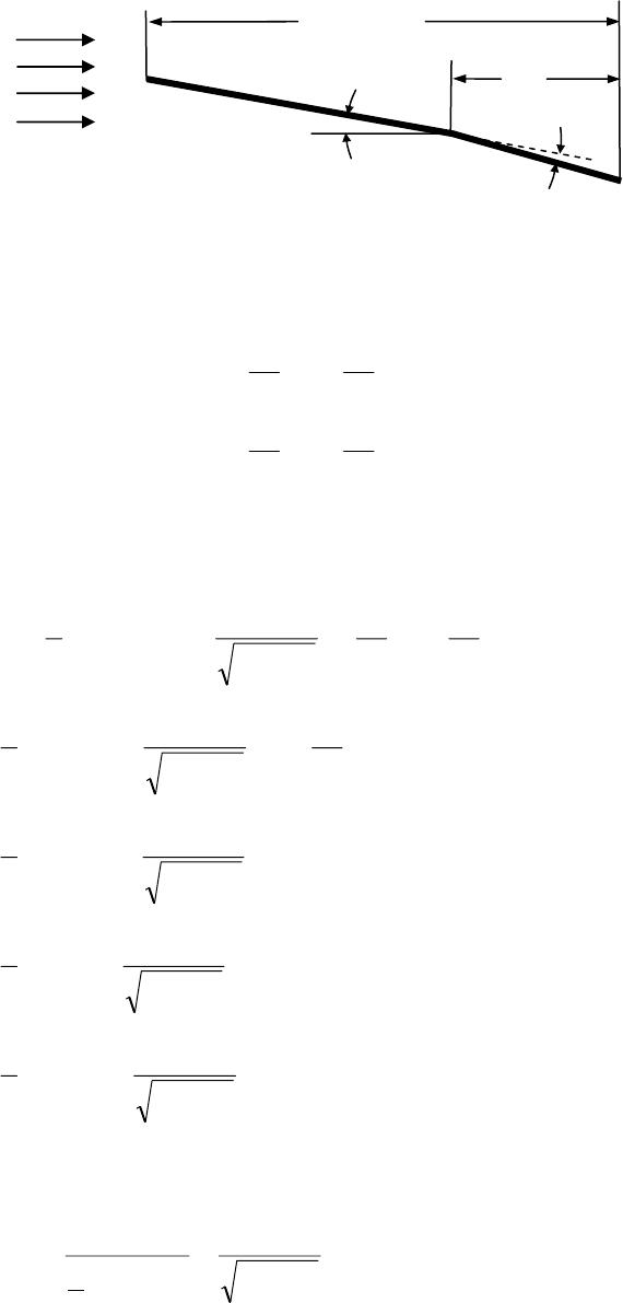
Problem 9. – Using thin airfoil theory, find CL and CD for a two-dimensional, flat plate

airfoil with deflected flap in supersonic flow of Mach number M∞. Plot CL versus α for

various δ for F=0.25 (Figure P13.9).

this material may be reproduced, in any form or by any means, without permission in writing from the publisher.

284

Figure P13.9

For the airfoil from Figure P13.9 we can distinguish two different regions:

()

cF1x0 −≤≤ α−=

⎟

⎠

⎞

⎜

⎝

⎛

=

⎟

⎠

⎞

⎜

⎝

⎛

ul dx

dy

dx

dy

()

cxcF1

≤

≤−

()

δ+α−=

⎟

⎠

⎞

⎜

⎝

⎛

=

⎟

⎠

⎞

⎜

⎝

⎛

ul dx

dy

dx

dy

We substitute these relations in the general expression of the lift for an airfoil

=

⎭

⎬

⎫

⎩

⎨

⎧⎟

⎠

⎞

⎜

⎝

⎛

+

⎟

⎠

⎞

⎜

⎝

⎛

⎟

⎠

⎞

⎜

⎝

⎛

−

−γ= ∫

∞

∞∞ dx

dx

dy

dx

dy

1M

2

Mp

2

1

L

ul

c

02

2

=

⎟

⎠

⎞

⎜

⎝

⎛

⎟

⎠

⎞

⎜

⎝

⎛

−

−γ ∫

∞

∞∞ dx

dx

dy

2

1M

2

Mp

2

1

l

c

0

2

()

[]

()

=

⎭

⎬

⎫

⎩

⎨

⎧δ+α−+α−

⎟

⎠

⎞

⎜

⎝

⎛

−

−γ ∫∫ −

−

∞

∞∞ c

cF1

0

2

2dxdx

1M

4

Mp

2

1

()( )

[]

=δ+α+−α

⎟

⎠

⎞

⎜

⎝

⎛

−

γ

∞

∞∞ FccF1

1M

4

Mp

2

1

2

()

F

1M

4

cMp

2

1

2

2δ+α

⎟

⎠

⎞

⎜

⎝

⎛

−

γ

∞

∞∞

Therefore, the lift coefficient CL is

()

F

1M

4

cMp

2

1

L

C2

2

Lδ+α

−

=

γ

=

∞

∞∞

Particularly, for F=0.25 CL is

Chord = c

Fc

α

δ

M∞

this material may be reproduced, in any form or by any means, without permission in writing from the publisher.

285

()

δ+α

−

=

∞

25.0

1M

4

C2

L

For the drag we get

=

⎥

⎦

⎤

⎢

⎣

⎡⎟

⎠

⎞

⎜

⎝

⎛

−

⎟

⎠

⎞

⎜

⎝

⎛

+

⎥

⎦

⎤

⎢

⎣

⎡⎟

⎠

⎞

⎜

⎝

⎛

+

⎟

⎠

⎞

⎜

⎝

⎛

⎟

⎠

⎞

⎜

⎝

⎛

−

γ= ∫∫ ∞

∞

∞∞ dx

dx

dy

dx

dy

pdx

dx

dy

dx

dy

1M

2

Mp

2

1

Dc

0lu

2

l

2

u

c

02

2

=

⎟

⎠

⎞

⎜

⎝

⎛

−

γ∫

∞

∞∞ dx

dx

dy

2

1M

2

Mp

2

12

l

c

0

2

()

=

⎟

⎠

⎞

⎜

⎝

⎛δ+α+α

−

γ∫∫ −

−

∞

∞∞ c

cF1

2

cF1

0

2

2dxdx

1M

4

Mp

2

1

()( )

[]

=δ+α+−α

−

γ

∞

∞∞ FccF1

1M

4

Mp

2

12

2

()

F2F

1M

4

cMp

2

122

2

2αδ+δ+α

−

γ

∞

∞∞

and the drag coefficient CD is

(

)

F2F

1M

4

cMp

2

1

D

C22

2

Dαδ+δ+α

−

=

γ

=

∞

∞∞

Consequently for F=0.25 CD is

()

αδ+δ+α

−

=

∞

5.025.0

1M

4

C22

2

D

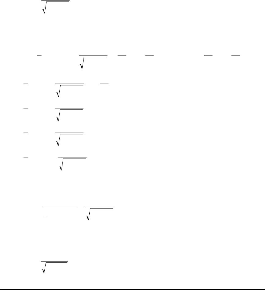
Problem 10. – Consider uniform supersonic flow over a wall in which there exists a

bump, as shown in Figure P13.10. Assuming linearized, two-dimensional potential flow,

calculate the vertical and horizontal components of the force on the bump. Assume M∞ =

2.0, with p∞ = 50 kPa.

this material may be reproduced, in any form or by any means, without permission in writing from the publisher.

286

Figure P13.10

For the wall from Figure P13.10 we can distinct two different regions where dxdy is

not zero

L5.0x0 ≤≤ 2.0

2

L

L1.0

dx

dy ==

LxL5.0 ≤≤ 2.0

2

L

L1.0

dx

dy −=−=

Using these relations in the general expression for the lift we get

=

⎟

⎠

⎞

⎜

⎝

⎛

⎟

⎠

⎞

⎜

⎝

⎛

−

−γ= ∫

∞

∞∞ dx

dx

dy

1M

2

Mp

2

1

LL

02

2

() ( )

0dx2.0dx2.0

1M

2

Mp

2

1L

L5.0

0

2

2=

⎥

⎦

⎤

⎢

⎣

⎡−+

⎟

⎠

⎞

⎜

⎝

⎛

−

−γ ∫∫

∞

∞∞

For the drag we can write

=

⎟

⎠

⎞

⎜

⎝

⎛

+

⎟

⎠

⎞

⎜

⎝

⎛

⎟

⎠

⎞

⎜

⎝

⎛

−

γ= ∫∫ ∞

∞

∞∞ dx

dx

dy

pdx

dx

dy

1M

2

Mp

2

1

Dc

0

2

c

02

2

() ( )

=

⎥

⎦

⎤

⎢

⎣

⎡−+

−

γ∫∫

∞

∞∞ L

L5.0

2

L5.0

0

2

2dx2.0dx2.0

1M

2

Mp

2

1

()

(

)

()

(

)

N66.6410104.0

12

2

10504.1L04.0

1M

M

p2

2

3

2

=⋅

−

⋅=

−

γ−

∞

M∞

p∞

L = 1 cm

0.5 0.5

0.1L

this material may be reproduced, in any form or by any means, without permission in writing from the publisher.

287

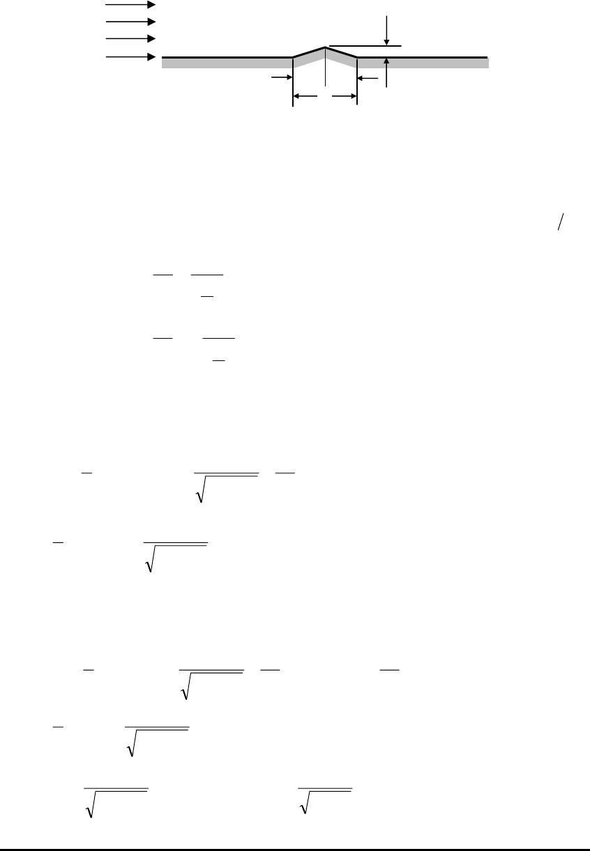
Problem 11. – A supersonic airfoil consists of a circular arc, as shown in Figure P13.11.

Compute the lift and drag coefficients of the foil versus angle of attack.

Figure P13.1l

The lift coefficient is

1M

4

C2

L−

α

=

∞

The airfoil with a shape of a circular arc has camber but no thickness, with

2.0

2

L

L1.0

dx

dC ==

Thus, the drag coefficient is

[]

=+α

−

=

⎥

⎦

⎤

⎢

⎣

⎡

⎟

⎠

⎞

⎜

⎝

⎛

+α

−

=

∞∞

22

2

D2.0

1M

4

dx

dC

1M

4

C

[]

04.0

1M

42

2+α

−

∞

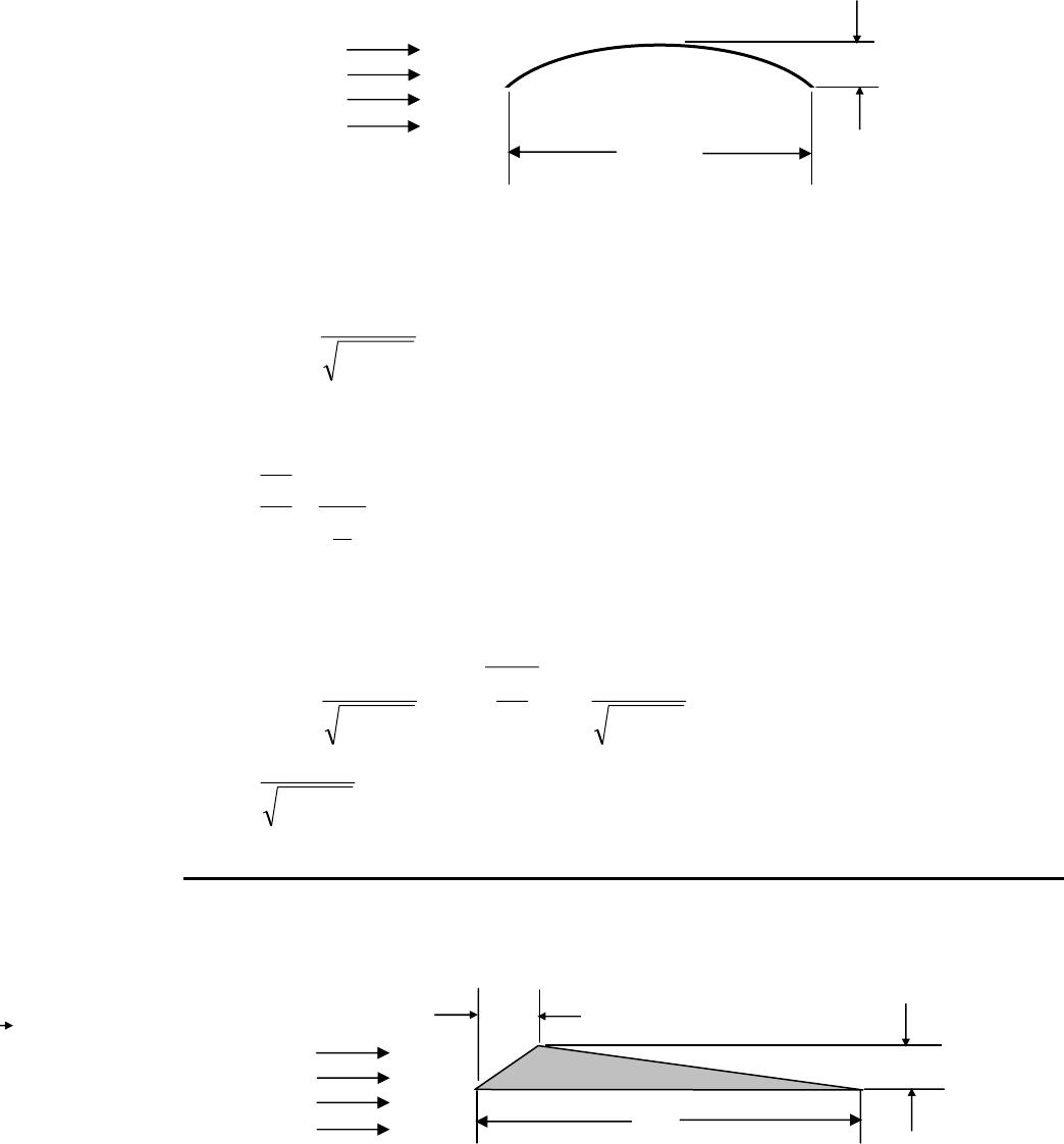
Problem 12. – For the airfoil shown in Figure P13.12, determine CL and CD versus angle

of attack in supersonic flow.

Figure P13.12

0.1L

M∞

L

0.08c

M∞

c

0.3c

this material may be reproduced, in any form or by any means, without permission in writing from the publisher.

288

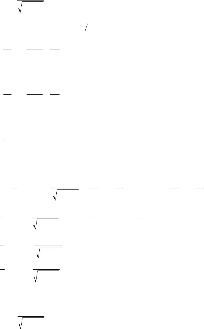
The lift coefficient is

1M

4

C2

L−

α

=

∞

For the upper surface of the airfoil, dxdy can have two distinctive values

3

8.0

c3.0

c08.0

dx

dy

u

==

⎟

⎠

⎞

⎜

⎝

⎛ for c3.0x0

≤

and

7

8.0

c7.0

c08.0

dx

dy

u

==

⎟

⎠

⎞

⎜

⎝

⎛ for cxc3.0

≤

For the lower surface of the airfoil

0

dx

dy

l

=

⎟

⎠

⎞

⎜

⎝

⎛

For zero angle of attack, the drag is

=

⎥

⎦

⎤

⎢

⎣

⎡⎟

⎠

⎞

⎜

⎝

⎛

−

⎟

⎠

⎞

⎜

⎝

⎛

+

⎥

⎦

⎤

⎢

⎣

⎡⎟

⎠

⎞

⎜

⎝

⎛

+

⎟

⎠

⎞

⎜

⎝

⎛

⎟

⎠

⎞

⎜

⎝

⎛

−

γ= ∫∫ ∞

∞

∞∞ dx

dx

dy

dx

dy

pdx

dx

dy

dx

dy

1M

2

Mp

2

1

Dc

0lu

2

l

2

u

c

02

2

=

⎥

⎦

⎤

⎢

⎣

⎡⎟

⎠

⎞

⎜

⎝

⎛−+

⎟

⎠

⎞

⎜

⎝

⎛

⎟

⎠

⎞

⎜

⎝

⎛

−

γ∫∫

∞

∞∞ c3.0

0

c

c3.0

22

2

2dx

7

8.0

dx

3

8.0

1M

2

Mp

2

1

=

⎟

⎠

⎞

⎜

⎝

⎛

−

γ

∞

∞∞ 03047.0

1M

2

cMp

2

1

2

1M

06095.0

cMp

2

1

2

−

γ

∞

∞∞

Consequently, for zero angle of attack, the drag coefficient is

1M

06095.0

C2

D−

=

∞

For an angle of attack α, we have an additional term

this material may be reproduced, in any form or by any means, without permission in writing from the publisher.

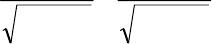
289

1M

06095.0

1M

4

C22

2

D−

+

−

α

=

∞∞

this material may be reproduced, in any form or by any means, without permission in writing from the publisher.