978-0131206687 Chapter 12 Part 1

250

Chapter Twelve

E

EX

XA

AC

CT

T

S

SO

OL

LU

UT

TI

IO

ON

NS

S

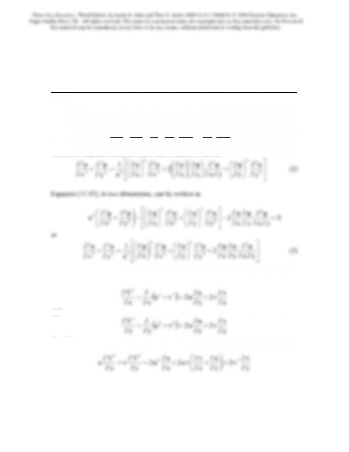
Problem 1. – The velocity potential equation can be written in a variety of forms. For

example, Taylor and Maccoll, Ref. 23, used the following forms for problems in

Cartesian coordinates

⎥

⎦

⎤

⎢

⎣

⎡

∂

⎟

⎠

⎞

⎜

⎝

⎛

∂

+

∂

⎟

⎠

⎞

⎜

⎝

⎛

∂

=

∂

+

∂

y

V

y

φ

x

V

x

φ

a

1

y

φ

x

φ22

22

2

(1)

Derive this expression and then show that it may be written as

⎥

⎤

⎢

⎡

∂

⎟

⎞

⎜

⎛

∂

+

∂

⎟

⎞

⎜

⎛

∂

⎟

⎞

⎜

⎛

∂

+

∂

⎟

⎞

⎜

⎛

∂

=

∂

+

∂

2

22

2

φ

2

φ

1

φ

φ (2)

⎥

⎦

⎢

⎣

∂∂

∂

⎟

⎠

⎜

⎝

∂

⎟

⎠

⎜

⎝

∂

yx

y

x

y

x

a

y

x

2

22

2

Note Eqs. (2) and (3) are identical. Further

()

x

v

v2

x

u

u2vu

xx

V22

2

∂

+

∂

=+

∂

=

∂

and

()

y

v

v2

y

u

u2vu

yy

V22

2

∂

+

∂

=+

∂

=

∂

therefore

y

v2

y

x

vu2

x

u2

y

v

x

u22

∂

+

⎟

⎠

⎜

⎝

∂

+

∂

+

∂

=

∂

+

∂

which leads to

this material may be reproduced, in any form or by any means, without permission in writing from the publisher.

⎟

⎠

⎞

⎜

⎝

⎛

∂

+

∂

−

⎟

⎠

⎞

⎜

⎝

⎛

∂

+

∂

=

∂

+

∂

y

u

x

v

vu

y

V

v

x

V

u

2

1

y

v

x

u

22

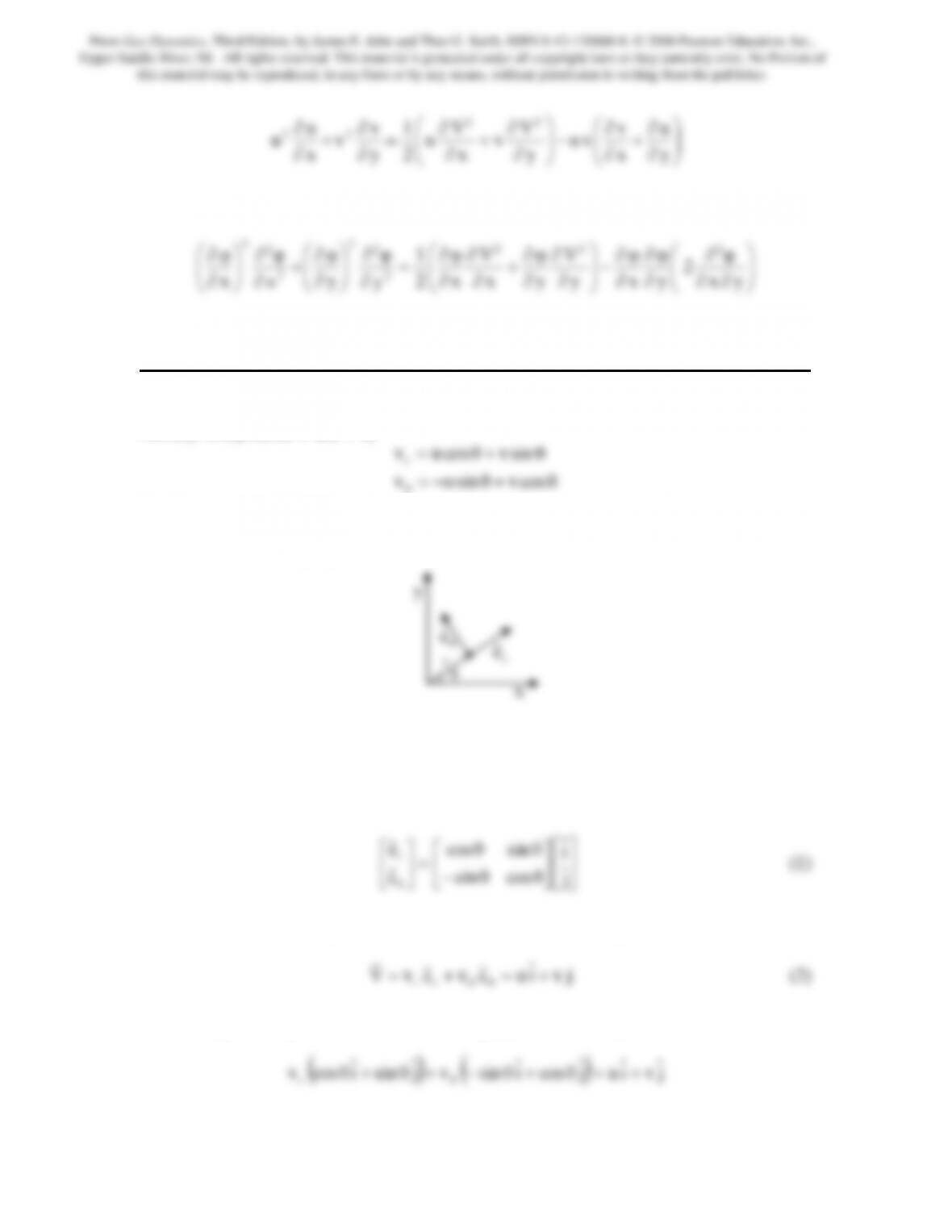
Using the definition of velocity potential, the above equation becomes

⎟

⎠

⎞

⎜

⎝

⎛

∂∂

∂

−

⎟

⎠

⎞

⎜

⎝

⎛

∂

+

∂

=

∂

⎟

⎠

⎞

⎜

⎝

⎛

∂

+

∂

⎟

⎠

⎞

⎜

⎝

⎛

∂

yx

φ

2

y

φ

x

φ

y

V

y

φ

x

V

x

φ

2

1

y

φ

y

φ

x

φ

x

φ2

22

2

Substitution of this into the right hand side of the Eq. (3) then yields Eq. (1).

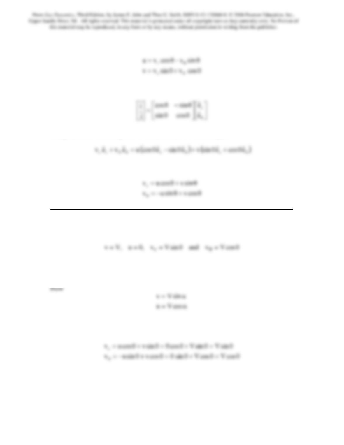
Problem 2. – Show that polar velocity components vr and vθ are related to the Cartesian

velocity components u and v by

θ+θ−=

θ

+

θ

=

θcosvsinuv

sinvcosuvr

Find the inverse of these, i.e., develop expressions for u = u (vr, vθ) and v = v (vr, vθ).

Consider the following figure

where r

e

ˆ and θ

e

ˆ are the unit normal vectors of the polar coordinate system. These unit

vectors are related to the Cartesian unit vectors, i

ˆand j

ˆ, through a counterclockwise

rotation of angle θ. In other words

⎥

⎦

⎢

⎣

⎥

⎦

⎢

⎣

θθ−

=

⎥

⎦

⎢

⎣

θj

ˆ

cossin

e

ˆ

Now consider the velocity vector expressed in both coordinate systems

Substituting for the polar unit vectors from Eq. (1) in the above yields

this material may be reproduced, in any form or by any means, without permission in writing from the publisher.

252

which after equating components gives

θ+θ=

θ

cosvsinvv

r

Taking the inverse of Eq. (1) leads to

⎥

⎦

⎤

⎢

⎣

⎡

⎥

⎦

⎤

⎢

⎣

⎡

θθ

=

⎥

⎦

⎢

⎣

θ

e

ˆ

cossin

j

ˆ

i

Using this and substituting for the Cartesian unit vectors in Eq.(2)

θ

+

θ

+

θ

−

θ

θθθθ

which after equating components gives

θ

+

θ

=

θ+θ−=

θcosvsinuv

Problem 3. – For a uniform flow in the +y direction, show that the expressions for the

velocity components in the previous problem give

θ

=

θ

=

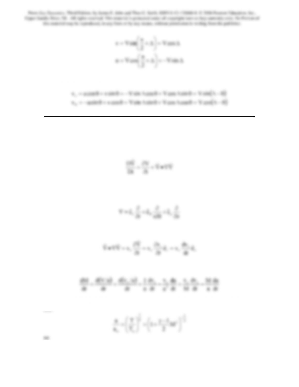
Obtain expressions for the velocity components for a uniform flow that is directed at an

angle π/2 + ∆.

α=

cosVu

at α = π/2, it is obvious that v = V and u = 0. Substituting these into the relations of the

previous problem produces

θ=θ+θ=θ+θ−=

θ

=

θ

+

θ

=

θ

+θ=

θcosVcosVsin0cosvsinuv

sinVsinVcos0sinvcosuvr

For a uniform flow that is directed at an angle of α = π/2 + ∆

this material may be reproduced, in any form or by any means, without permission in writing from the publisher.

θ

−

θ

=

∆−=

⎟

⎠

⎞

⎜

⎝

⎛∆+

π

=

∆=

⎟

⎠

⎞

⎜

⎝

⎛∆+

π

=

sinV

2

cosVu

cosV

2

sinVv

Substituting these into the relations of the previous problem produces

()

θ−∆=θ∆+θ∆=θ+θ−=

θcosVcoscosVsinsinVcosvsinuv

Problem 4. – Prove that as the limit line for radial flow is approached the acceleration of

the flow approaches ∞.

Flow acceleration is composed of an unsteady and convection terms

t

D

t

∂

Since the flow is steady and purely radial ∂V/∂t = 0 and rr e

ˆ

vV =

r

. In cylindrical

coordinates

r

Now

r

rr

rr e

d

r

∂

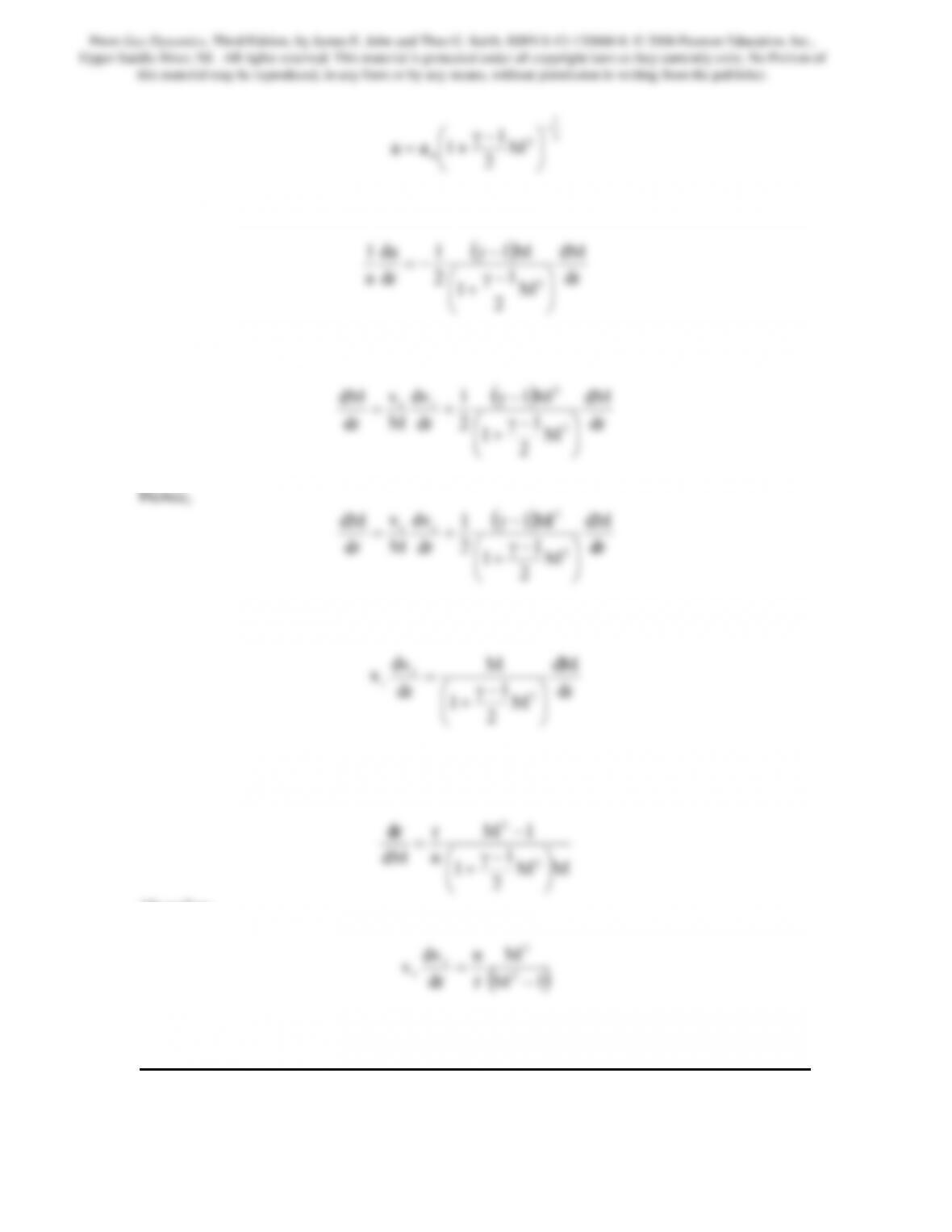
The radial derivative of the Mach number is

d

r

a

d

r

M

d

r

a

d

r

a

d

r

d

r

d

r

2

But

1

this material may be reproduced, in any form or by any means, without permission in writing from the publisher.

254

1

oM

2

−

⎠

⎝

Take the logarithmic derivative of this to get

dr

M

2

1

2

dr

a

2⎟

⎠

⎞

⎜

⎝

⎛−γ

+

Insert this into the expression for the radial derivative of the Mach number and obtain

dr

M

2

1

2

dr

M

dr

2

⎟

⎠

⎞

⎜

⎝

⎛−γ

+

dr

M

2

1

2

dr

M

dr

2

⎟

⎠

⎞

⎜

⎝

⎛−γ

+

Rearranging gives

dr

M

2

1

dr

2

r

⎟

⎠

⎞

⎜

⎝

⎛−γ

+

The radial derivative of the Mach number can also be obtained from Eq.(12. 7), i.e.,

MM

2

1

n

dM

2

⎟

⎠

⎞

⎜

⎝

⎛−γ

+

Therefore,

()

1M

r

dr

r−

As r → r* M→ 1, hence, the convective acceleration is infinite.

this material may be reproduced, in any form or by any means, without permission in writing from the publisher.

255

Problem 5. – Starting from the concept that the streamlines are straight for radial flow

and therefore have the form ψ = cθ = ctan−1(y/x), develop an equation for the velocity

field of a compressible fluid.

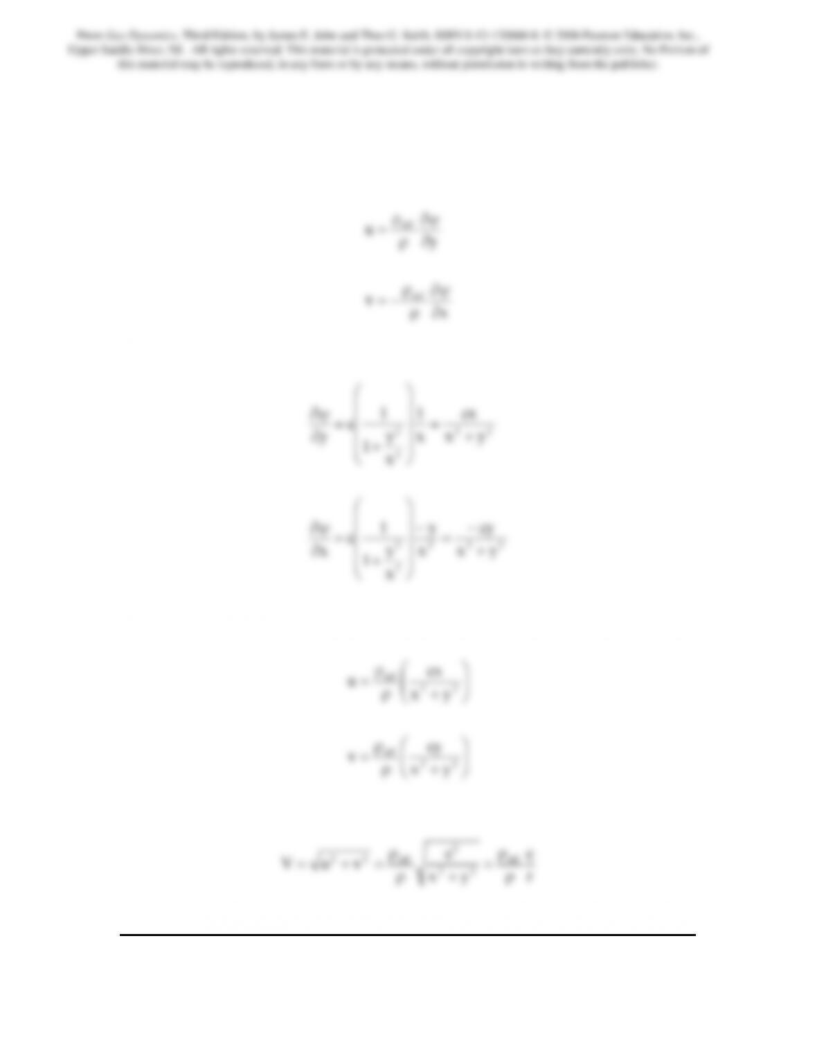
As defined in Problem 11.3

x

v

ref

∂

ψ∂

ρ

−=

Now ψ = ctan−1(y/x), so

222

2

yx

cy

x

y

x

y

1

c

x

+

−

=

−

⎟

⎠

⎞

⎜

⎝

⎛

+

=

∂

ψ∂

So the velocity components are

⎟

⎠

⎞

⎜

⎝

⎛

+

ρ

=

22

ref

yx

cy

v

Hence,

r

yx

22

ρ

+

ρ

this material may be reproduced, in any form or by any means, without permission in writing from the publisher.

Problem 6. – Sketch the ellipse of Eq.(12.13) in the first quadrant. Indicate roughly

subsonic and hypersonic regimes. Use the sketch to explain which effect, thermodynamic

or inertial, dominates in subsonic and hypersonic accelerations.

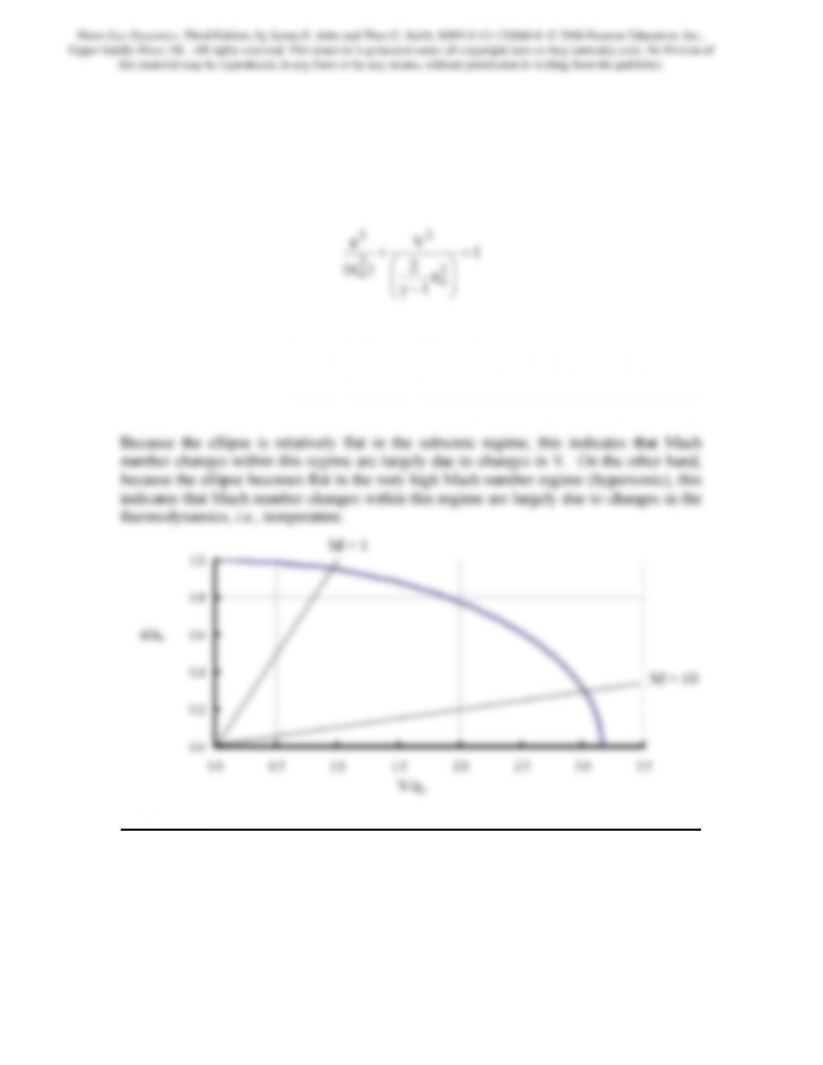
Equation (12.13)

a

1

2

)a(

2

o

2

o

⎟

⎠

⎞

⎜

⎝

⎛

−γ

is plotted for a γ = 1.4 in the figure below. The y axis may be regarded as the

thermodynamic axis since it contains the speed of sound ratio a/ao. The x axis may be

regarded as the kinematic axis since it contains the speed ratio V/ao. Lines for two Mach

numbers are shown on the plot. To the left of the M =1 line the flow is subsonic; to the

right supersonic.

this material may be reproduced, in any form or by any means, without permission in writing from the publisher.

257

1

2

o

1

2

o

2

o

M

2

1

2

1

p

M

2

1

T

−γ

γ

⎟

⎠

⎞

⎜

⎝

⎛−γ

+=

ρ

⎠

⎞

⎝

⎛−γ

−γ

+=

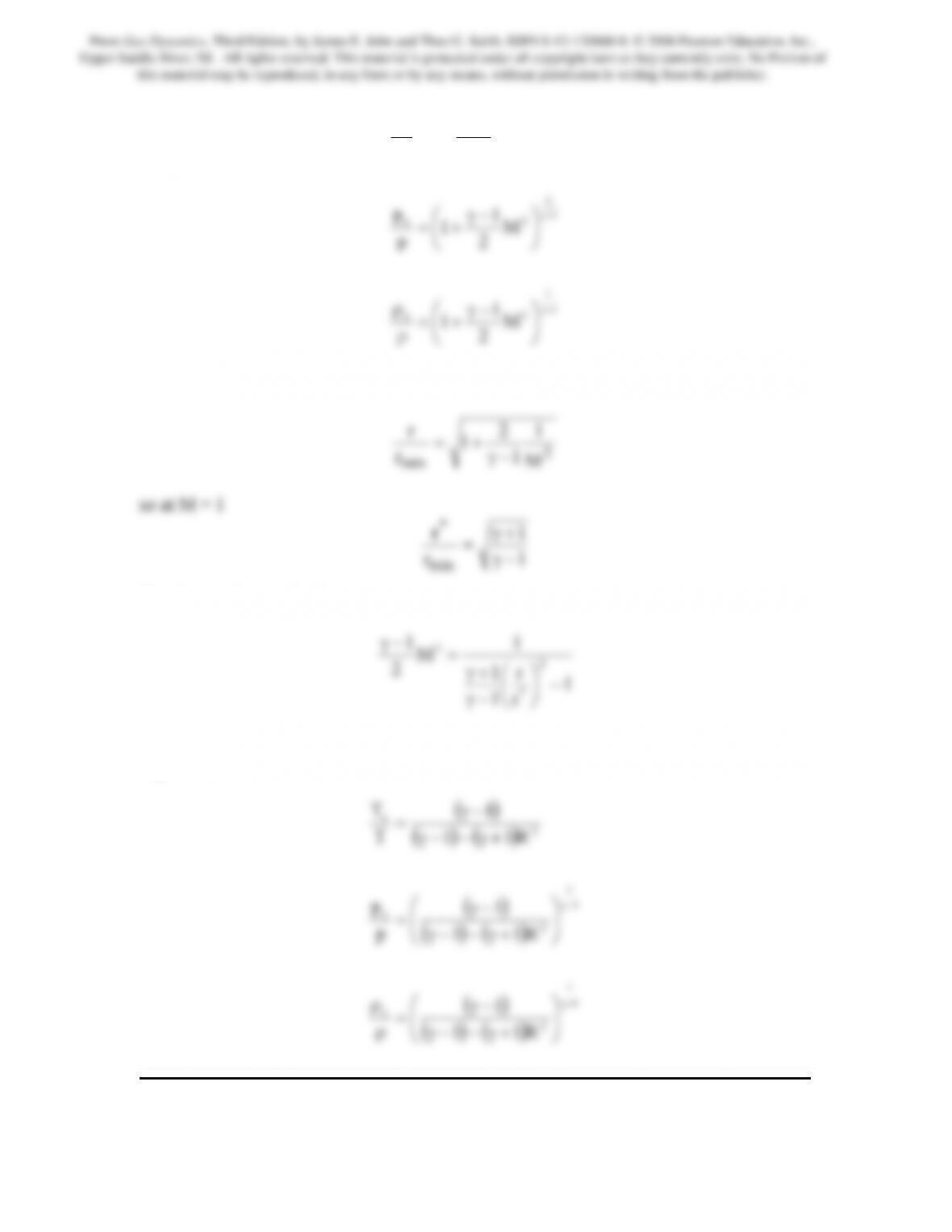
For the irrotational compressible vortex we have shown [Eq.(12.16)] that

Combining these and solving gives

1

r

1

2

*

−

⎟

⎠

⎞

⎜

⎝

⎛

−γ

+γ

Replacing this term in each of the ratios and defining R = r/r* produces the desired

expressions

()()

()

()()

1

2

o

2

R11

1

R11

p

−γ

⎟

⎠

⎞

⎜

⎝

⎛

+γ−−γ

−γ

=

ρ

⎟

⎠

⎜

⎝

+γ−−γ

this material may be reproduced, in any form or by any means, without permission in writing from the publisher.

258

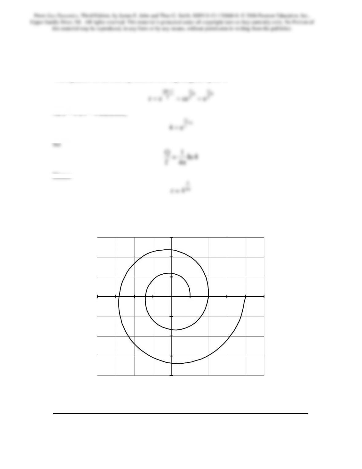
Problem 8. – Plot the incompressible flow equiangular spiral from θ = 0 to θ = 4 π.

Assume that the constant c is unity, i.e., C = 0. Select the ratio of Q/Γ so that r = 4 at

θ = 4π.

The equation for an incompressible flow equiangular spiral is

The corresponding x and y coordinates are x = rcosθ and y = rsinθ. A plot of these with

θ as the parameter provides the following

-4

-3

-2

-1

0

1

2

3

-4 -3 -2 -1 0 1 2 3 4 5

this material may be reproduced, in any form or by any means, without permission in writing from the publisher.

259

Problem 9. – Use the hodograph transformation to obtain a solution for the case in which

ψ = ψ(V). Show that for this case φ = cα.

Elimination of the velocity potential from the Chaplygin-Molenbroek equations,

Eqs.(12.52) and (12.53) was shown to produce

0

a

1

V

V2

2

α∂

⎟

⎠

⎜

⎝

ρ

+

⎟

⎠

⎜

⎝

∂

ρ

∂

Since for this problem ψ = ψ(V), this expression reduces to

0

dV

V

dV

⎟

⎠

⎜

⎝

ρ

Integration brings

C

dV

V

o=

ρ

But from Eq.(12.52)

C

dV

d

V

o=

ψ

ρ

=

α∂

φ∂

Problem 10. – Another method to obtain the hodograph equations is to make use of the

Legrendre transformation, Zwillinger, Ref. 24. In this approach a function, Φ(u,v), in

the hodograph plane is related to the velocity potential, φ(x,y), by

Use this relation to show that

(a) x

u=

∂

v=

∂

this material may be reproduced, in any form or by any means, without permission in writing from the publisher.

260

22

2

1

v

J

1

x

Φ∂

φ∂

∂

Φ∂

=

∂

φ∂

vvuv

(c) Finally, show that Eq.(12.27) is transformed into the following linear equation

0

ua

v

1

vu

a

uv

2

va

u

12

2

22

2

∂

Φ∂

⎟

⎠

⎜

⎝

∂∂

Φ∂

+

∂

Φ∂

⎟

⎠

⎜

⎝

(a) Differentiate )y,x(yvxu φ−+=Φ with respect to u and obtain

u

yu

xu

vx

u

u∂

∂

−

∂

−

∂

++

∂

=

∂

But from the definition of the velocity potential u

x=

∂

φ

∂

and v

y=

∂

φ

∂

, so the above

reduces to

∂

φ

∂

φ

Similarly differentiate )y,x(yvxu

φ

−

+=Φ with respect to v and obtain

∂

φ

∂

φ

(b) Differentiate ∂Φ/∂u = x first with respect to u and also with respect to v to obtain

=

Φ

vuv

Similarly using ∂Φ/∂v = y we obtain

this material may be reproduced, in any form or by any means, without permission in writing from the publisher.