Fluid Mechanics, 6th Ed. Kundu, Cohen, and Dowling
Exercise 9.41. Consider the development from rest of plane Couette flow. The flow is bounded
by two rigid boundaries at y = 0 and y = h, and the motion is started from rest by suddenly
accelerating the lower plate to a steady velocity U. The upper plate is held stationary. Here a
similarity solution cannot exist because of the appearance of the parameter h. Show that the
velocity distribution is given by
u(y,t)=U1−y
h
#
$
% &
‘
( −2U
π
1
nexp −n2
π
2
ν
t
h2
#
$
% &
‘
(
n=1
∞
∑sin n
π
y
h
#
$
% &
‘
(
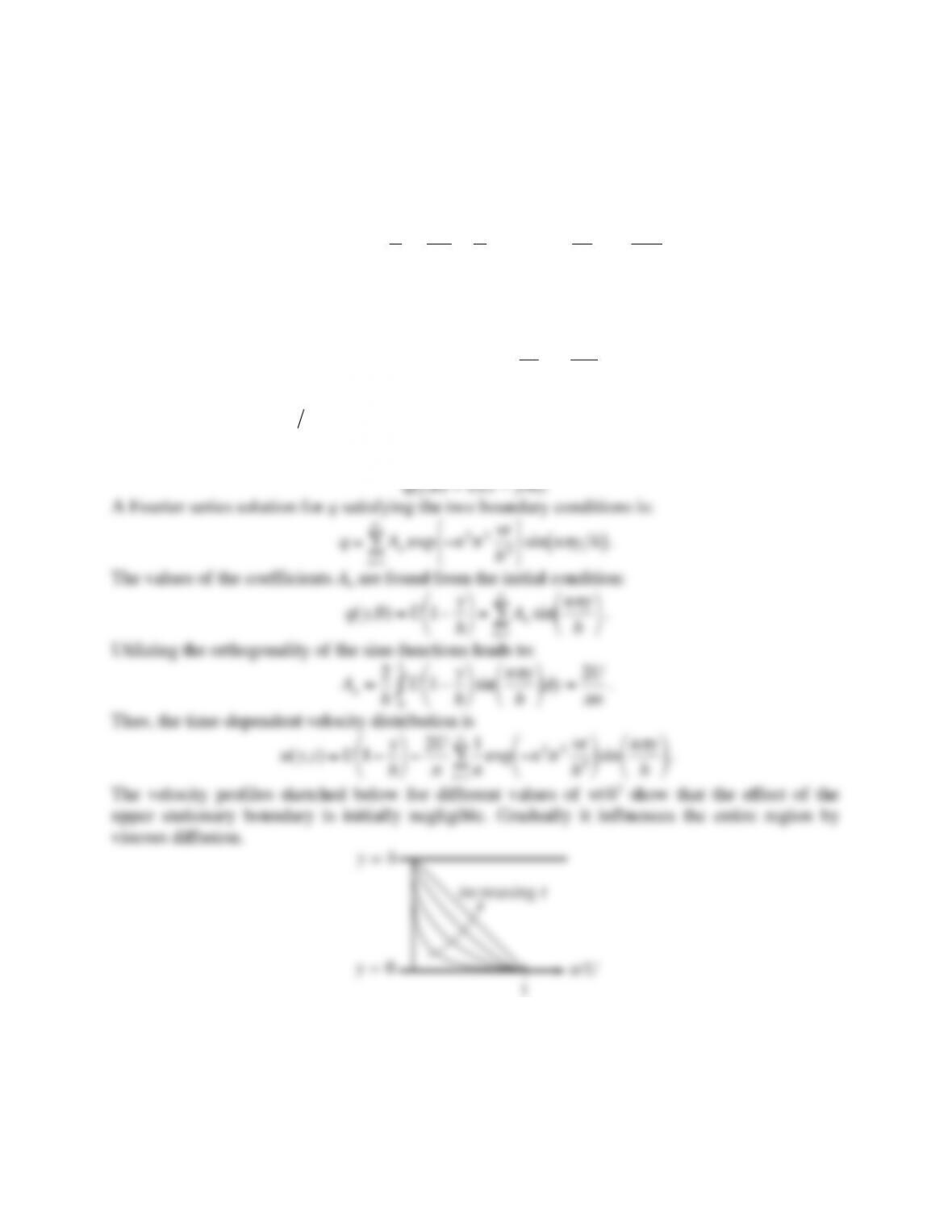
Sketch the flow pattern at various times, and observe how the velocity reaches the linear
distribution for large times.
Solution 9.41. The differential equation is (9.20),
∂
u
∂
t=
ν∂
2u
∂
y2
, and the boundary and initial
conditions on u(y,t) are: u(0,t) = U, u(h,t) = 0, and u(y,0) = 0. The solution is facilitated by
defining
u(y,t)=U1−y h
( )
+q(y,t)
, where q is the deviation of the velocity from the final linear
distribution. The deviation velocity satisfies the same differential equation, but with
homogeneous boundary conditions: q(0,t) = q(h,t) = 0, and the initial condition:
q(y,0) = U(1 – y/h).
#
$
% &
‘
( −2U
1
2
ν
t
#
$
% &
‘
(
n=1
∞
∑sin n
π
y
h
#
$
% &
‘
(
Fluid Mechanics, 6th Ed. Kundu, Cohen, and Dowling
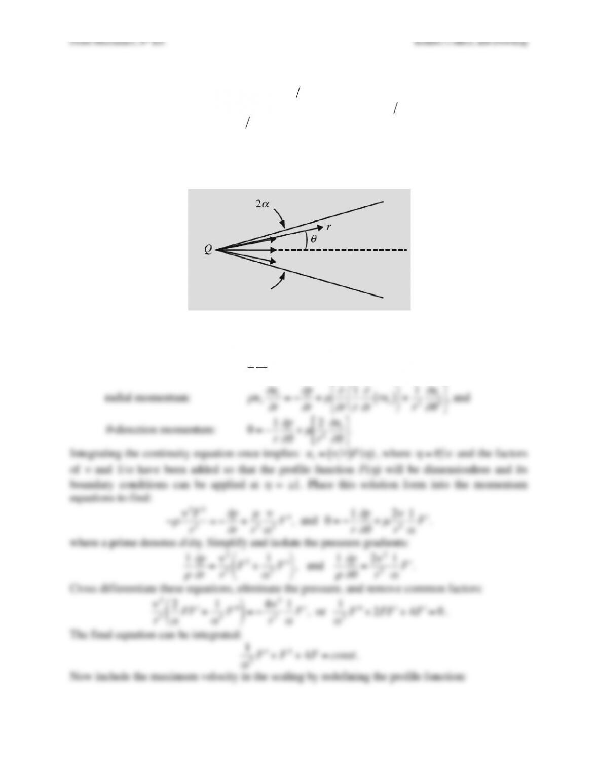
Exercise 9.42. Two-dimensional flow between flat non-parallel plates can be formulated in
terms of a normalized angular coordinate,
η
=
θ α
, where
α
is the half angle between the plates,
and a normalized radial velocity,
ur(r,
θ
)=umax (r)f(
η
)
where
η
=
θ α
for |
θ
| ≤
α
. Here, u
θ
= 0,
the Reynolds number is
Re =umax r
α ν
, and Q is the volume flux (per unit width perpendicular
to the page).
a) Using the appropriate versions of (4.10) and (8.1), show that
“ “
f +Re
α
f2+4
α
2f=const.
b) Find f(
η
) for symmetric creeping flow, i.e.
Re =0=f(+1) =f(−1)
, and f(0) = 1.
c) Above what value of the channel half-angle will backflow always occur?
Solution 9.42. a) In two-dimensional (r,
θ
)-polar coordinates, the governing equations for steady
radial flow,
ur(r,
θ
)=umax (r)f(
η
)
, are:
continuity:
1
r
∂
∂
r
rur
( )
=0
,
radial momentum:
ρ
ur
∂
ur
∂
r=−
∂
p
∂
r+
µ∂
∂
r
1
r
∂
∂
rrur
( )
%
&
‘ (
)
* +1
r2
∂
ur
∂θ
2
,
.
/
1
η
=
θ α
, and
Fluid Mechanics, 6th Ed. Kundu, Cohen, and Dowling
Fluid Mechanics, 6th Ed. Kundu, Cohen, and Dowling
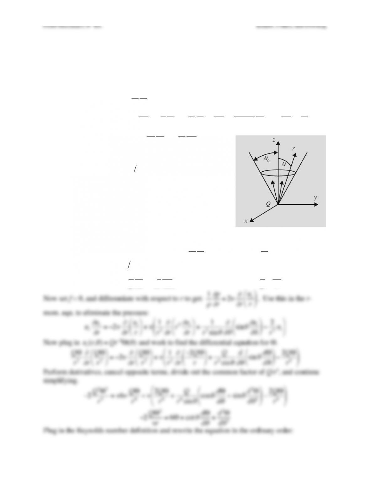
Exercise 9.43. Consider steady viscous flow inside a cone of constant angle
θ
o. The flow has
constant volume flux = Q, and the fluid has constant density =
ρ
and constant kinematic viscosity
=
ν
. Use spherical coordinates, and assume that the flow only has a radial component,
u=ur(r,
θ
),0,0
( )
which is independent of the azimuthal angle
ϕ
, so that the equations of motion
are:
Cons. of Mass:
1
r2
∂
∂
r
r2ur
( )
=0
Cons. of Radial Mom.:
ur
∂
ur
∂
r=−1
ρ
∂
p
∂
r+
ν
1
r2
∂
∂
rr2
∂
ur
∂
r
&
‘
( )
*
+ +1
r2sin
θ
∂
∂θ
sin
θ∂
ur
∂θ
&
‘
( )
*
+ −2
r2ur
&
‘
(
)
*
+
Cons. of
θ
-Mom.
0=−1
ρ
r
∂
p
∂θ
+
ν
2
r2
∂
ur
∂θ
‘
(
) *
+
,
For the following items, assume the radial velocity can be
determined using:
ur(r,
θ
)=QR(r)Θ(
θ
)
. Define the Reynolds
number of this flow as: Re =
Q(
πν
r)
.
a) Use the continuity equation to determine R(r).
b) Integrate the
θ
-momentum equation, assume the constant of
integration is zero, and combine the result with the radial mom.
equ. to determine a single differential equation for Θ(
θ
) in
terms of
θ
and Re. It is not necessary to solve this equation.
c) State the matching and/or boundary conditions that Θ(
θ
)
must satisfy.
Solution 9.43. a) Place
ur(r,
θ
)=QR(r)Θ(
θ
)
into
1
r2
∂
∂
r
r2ur
( )
=0
, to find:
∂
∂
r
r2R
( )
=0
for r ≠ 0.
Thus: r2R = constant or
R∝1r2
, so
ur(r,
θ
)=Qr−2Θ(
θ
)
, so Θ is a dimensionless function.
b) Rewrite the
θ
-mom. equ.:
1
ρ
∂
p
∂θ
=
ν
2
r
∂
ur
∂θ
&
‘
( )
*
+
, integrate with respect to
θ
:
p
ρ
=2
ν
rur+f(r)
.
Now set f = 0, and differentiate with respect to r to get:
1
ρ
∂
p
∂
r=2
ν∂
∂
r
ur
r
%
&
‘ (
)
*
. Use this in the r–
ur(r,
θ
θ
)
Fluid Mechanics, 6th Ed. Kundu, Cohen, and Dowling
Fluid Mechanics, 6th Ed. Kundu, Cohen, and Dowling
Exercise 9.44. The boundary conditions on obstacles in Hele-Shaw flow were not considered in
Example 9.4. Therefore, consider them here by examining Hele-Shaw flow parallel to a flat
obstacle surface at y = 0. The Hele-Shaw potential in this case is:
φ
=Ux z
h
1−z
h
“
#
$%
&
‘
,
where (x, y, z) are Cartesian coordinates and the flow is confined to 0 < z < h and y > 0.
a) Show that this potential leads to a slip velocity of
u(x,y→0) =U z h
( )
1−z h
( )
, and determine
the pressure distribution implied by this potential.
b) Since this is a viscous flow, the slip velocity must be corrected to match the genuine no-slip
condition on the obstacle’s surface at y = 0. The analysis of Example (9.4) did not contain the
correct scaling for this situation near y = 0. Therefore, rescale the x-component of (9.1) using:
x* = x/L, y* = y/h = y/
ε
L, z* = z/h = z/
ε
L, t* = Ut/L, u* = u/U, v* = v/
ε
U, w* = w/
ε
U, and p* = p/Pa,
and then take the limit as
ε
2ReL → 0, with
µ
UL/Pah2 remaining of order unity, to simplify the
resulting dimensionless equation that has
0≅dp
dx +
µ∂
2u
∂
y2+
∂
2u
∂
z2
“
#
$%
&
‘
as its dimensional counterpart.
c) Using boundary conditions of u = 0 on y = 0, and
u=U z h
( )
1−z h
( )
for y >> h. Show that
u(x,y,z)=Uz
h1−z
h
“
#
$%
&
‘+Ansin n
π
hz
“
#
$%
&
‘
n=1
∞
∑exp −n
π
hy
“
#
$%
&
‘
, where
An=−2U
h
z
h
1−z
h
“
#
$%
&
‘sin n
π
h
z
“
#
$%
&
‘
0
h
∫dz
,
which implies:
An=−8U n3
π
3
for n = odd, and An = 0 for n = even. [The results here are directly
applicable to the surfaces of curved obstacles in Hele-Shaw flow when the obstacle’s radius of
curvature is much greater than h.]
Solution 9.44. a) From Example 9.4, the u and v velocity components implied by the given
potential are:
u=
∂
∂
x
φ
=Uz
h
1−z
h
%
&
‘ (
)
*
and
v=
∂
∂
y
φ
=0
.
Neither of these equations shows any dependence on y, so, as
y→0
, the velocity components
Fluid Mechanics, 6th Ed. Kundu, Cohen, and Dowling
c) The field equation derived in part b) for u is linear. Therefore assume that it can be written as
a sum of two terms, one that provides the correct behavior when y >> h and one that acts to
provide the correct boundary condition at y = 0:
u=Uz
h1−z
h
#
$
% &
‘
( +
υ
(y,z)
, (i)
where
υ
= 0 when z = 0 and z = h,
υ
→0
when y >> h, and
u→0
when
y→0
. Using –∂p/∂x =
2
µ
U/h2, the part b) field equation becomes:
1
ρ
2
µ
U
h2+
ν
−2U
h2
%
&
‘ (
)
* +
ν∂
2
υ
∂
y2+
∂
2
υ
∂
z2
%
&
‘
(
)
* =0
, or
∂
2
υ
∂
y2+
∂
2
υ
∂
z2=0
.
Thus,
υ
solves a two dimensional Laplace equation. Here, a separation of variable solution,
υ
υ
(y, z) takes the following form:
υ
(y,z)=Ansin knz
( )
exp −kny
{ }
n=1
∞
∑
. (ii)
to allow for all possible values of k. To satisfy the final boundary condition (
u→0
when
y→0
Fluid Mechanics, 6th Ed. Kundu, Cohen, and Dowling
Fluid Mechanics, 6th Ed. Kundu, Cohen, and Dowling
Exercise 9.45. Using the velocity field (8.49), determine the drag on Stokes’ sphere from the
surface pressure and the viscous surface stresses
σ
rr and
σ
r
θ
.
Solution 9.45. There are pressure and shear stress contributions to the drag on a moving sphere
at low Reynolds number. The pressure distribution is given by (8.50):
p(r,
θ
)−p∞=−3
µ
aU
2r2cos
θ
.
The pressure drag can be obtained by integrating this result:
Fpressure =−p(r=a,
θ
)er⋅ezdS =−2
π
a2
µ
3U
2a
&
‘
( )
*
+
cos2
θ
θ
=0
θ
=
π
∫
surface
∫sin
θ
d
θ
=2
πµ
Ua
The viscous drag can be obtained from surface integrals of the viscous stresses:
Fvicous =−
σ
r
θ
(r=a,
θ
)e
θ
⋅ezdS +
σ
rr (r=a,
θ
)er⋅ezdS
surface
∫
surface
∫
=−2
π
a2
σ
r
θ
(r=a,
θ
)sin2
θ
d
θ
θ
=0
θ
=
π
∫+2
π
a2
σ
rr (r=a,
θ
)cos
θ
sin
θ
d
θ
θ
=0
θ
=
π
∫,
where
σ
r
θ
=
µ
1
r
∂
ur
∂θ
+
∂
u
θ
∂
r−u
θ
r
&
‘
( )
*
+ =−
µ
Usin
θ
r
3a3
2r3
&
‘
(
)
*
+
, and
σ
rr =2
µ∂
ur
∂
r=2
µ
Ucos
θ
3a
2r2−3a3
2r4
&
‘
(
)
*
+
.
Thus, at r = a,
σ
r
θ
≠ 0, but
σ
rr = 0, so
Fvicous =3
πµ
Ua sin3
θ
d
θ
θ
=0
θ
=
π
∫=4
πµ
Ua
.
Thus, one third of the drag comes from pressure forces and two thirds come from the shear
stress. The total drag is the sum of these two contributions:
Fdrag =Fpressure +Fvicous =2
πµ
Ua +4
πµ
Ua =6
πµ
Ua
.
Fluid Mechanics, 6th Ed. Kundu, Cohen, and Dowling
Exercise 9.46. Calculate the drag on a spherical droplet of radius r = a, density
ρ
) and viscosity
µ
) moving with velocity U in an infinite fluid of density
ρ
and viscosity
µ
. Assume Re =
ρ
Ua/
µ
<< 1. Neglect surface tension.
Solution 9.46. The effort here is similar to that in Section 8.6 for low Reynolds number flow past
a sphere. The main difference being that flow inside and outside the sphere must be considered
simultaneously. In the following solution, dimensionless variables are used without any special
notation. These are: ur/U, u
θ
/U, r/a,
ψ
/(Ua2), (p – p∞)/(
µ
U/a), and
τ
/(
µ
U/a), so that the surface of
the sphere is r = 1, and the free stream speed is unity. The development leading to (8.48)
suggests that the flow outside the sphere can be determined from:
ψ
o=Aor4+Bor2+Cor+Dor
( )
sin2
θ
for r > a.
To recover a uniform flow far from the sphere, the first two constants must be A = 0 and B = 1/2.
Similarly, the flow inside the sphere can be represented by
ψ
i=Air4+Bir2+Cir+Dir
( )
sin2
θ
for r < a.
Here, Di = 0 to avoid a singularity at r = 0.
Compute the velocities inside and outside the sphere:
ur=−1
r2sin
θ
∂ψ
∂θ
=
−2cos
θ
1
2+Co
r+Do
r3
&
‘
( )
*
+
for r>1
−2cos
θ
Air2+Bi+Ci
r
&
‘
( )
*
+
for r<1
,
–
.
.
/
.
.
0
1
.
.
2
.
.
, and
u
θ
=1
rsin
θ
∂ψ
∂
r=
sin
θ
1+Co
r−Do
r3
&
‘
( )
*
+
for r>1
sin
θ
4Air2+2Bi+Ci
r
&
‘
( )
*
+
for r<1
,
–
.
.
/
.
.
0
1
.
.
2
.
.
.
For a bounded velocity inside the sphere, Ci must be 0. There are four remaining boundary and
matching conditions at r = 1:
ur(1+) = 0 and ur(1–) = 0, and these imply
1
2+Co+Do=0
, and
Ai+Bi=0
; (1,2)
u
θ
(1+) = u
θ
(1–), and this implies
1+Co−Do=4Ai+2Bi
; and (3)
the stress continuity condition:
Fluid Mechanics, 6th Ed. Kundu, Cohen, and Dowling
In the following, force is made dimensionless by
µ
Ua, area is made dimensionless with a2, and
stress is made dimensionless with
µ
U/a. The normal and surface elements are:
The
θ
-component of surface shear stress
e
θ
6(Do/a3)sin2
θ
d
θ
d
ϕ
=e
θ
3
2
$
µ
µ
+$
µ
sin
θ
d
θ
d
ϕ
.
The r-component includes a pressure contribution which must be found by integrating Stokes’
creeping-flow momentum equation:
Thus, the r-component of the force integrand is:
−p+2
∂
ur
∂
r
$
%
& ‘
(
)
err2sin
θ
d
θ
d
ϕ
[ ]
r=1
,
–
.
/
0
1 =−3
2
cos
θ
2
µ
+2
µ
2
µ
+
µ
ersin
θ
d
θ
d
ϕ
.
So, the force on the liquid sphere is:
F=−er
3
2
cos
θ
$
µ
+2
µ
$
µ
+
µ
+e
θ
3
2
$
µ
µ
+$
µ
%
&
‘
(
)
*
ϕ
=0
2
π
∫
θ
=0
π
∫sin
θ
d
θ
d
ϕ
.
The unit vectors on the surface of the sphere are functions of the polar and azimuthal angles,
θ
,
ϕ
, respectively. They must be put in terms of the Cartesian unit vectors that do not vary with
position. The necessary relationships are:
er=excos
ϕ
sin
θ
+eysin
ϕ
sin
θ
+ezcos
θ
, and
e
θ
=excos
ϕ
cos
θ
+eysin
ϕ
cos
θ
−ezsin
θ
.
Integrating first over j, the x– and y-direction contributions to the force are zero, a result that can
also be deduced from the axial symmetry of the flow. This leaves:
F=2
π
ez−3
2
$
µ
+2
µ
$
µ
+
µ
cos2
θ
sin
θ
−3
2
$
µ
µ
+$
µ
sin3
θ
&
‘
(
)
*
+
θ
=0
π
∫d
θ
.
Carrying out the trigonometric integrals leads to:
Fluid Mechanics, 6th Ed. Kundu, Cohen, and Dowling
Fluid Mechanics, 6th Ed. Kundu, Cohen, and Dowling
Exercise 9.47. Consider a very low Reynolds number flow over a circular cylinder of radius r =
a. For r/a = O(1) in the Re = Ua/
ν
→ 0 limit, find the equation governing the stream function
ψ
(r,
θ
) and solve for
ψ
with the least singular behavior for large r. There will be one remaining
constant of integration to be determined by asymptotic matching with the large r solution (which
is not part of this problem). Find the domain of validity of your solution.
Solution 9.47. The Stokes’ flow field equation is:
∇p=
µ
∇2u
,
which can be rewritten:
∇p=−
µ
∇ × ∇ × u
.
Applying one more curl, eliminates the pressure gradient:
0=∇ × ∇ × ∇ × u
.
In two-dimensional (r,
θ
)-polar coordinates, the relationship between the stream function
ψ
(r,
θ
)
and the velocity field is
u=−ez× ∇
ψ
, so the field equation for the stream function is given by:
0=∇ × ∇ × ∇ × −ez× ∇
ψ
( )
.
This relationship can be converted to coordinate specific derivatives in steps. Start with the
stream function definition.
−ez× ∇
ψ
=1
r
∂ψ
∂θ
er−
∂ψ
∂
r
e
θ
Apply the first curl operation, using the formulae in Appendix B:
∇ × −ez× ∇
ψ
( )
=−ez
1
r
∂
∂r
r∂
ψ
∂r
‘
(
) *
+
, +1
r2
∂2
ψ
∂
θ
2
.
/
0
1
2
3
.
Apply the second curl operation,
∇ × ∇ × −ez× ∇
ψ
( )
=−er
1
r
∂
∂θ
1
r
∂
∂r
r∂
ψ
∂r
(
)
* +
,
– +1
r2
∂2
ψ
∂
θ
2
.
/
0
1
2
3
+e
θ
∂
∂
r
1
r
∂
∂r
r∂
ψ
∂r
(
)
* +
,
– +1
r2
∂2
ψ
∂
θ
2
.
/
0
1
2
3
.
Apply third and final curl operation,
0=∇ × ∇ × ∇ × −ez× ∇
ψ
( )
=
ez
1
r
∂
∂r
r
∂
∂
r
1
r
∂
∂r
r∂
ψ
∂r
‘
(
) *
+
, +1
r2
∂2
ψ
∂
θ
2
.
/
0
1
2
3
‘
(
)
*
+
, +1
r2
∂
∂θ
2
1
r
∂
∂r
r∂
ψ
∂r
‘
(
) *
+
, +1
r2
∂2
ψ
∂
θ
2
.
/
0
1
2
3
4
5
6
7
6
8
9
6
:
6
.
For large r, ur ~ cos
θ
, and u
θ
~ –sin
θ
, so it is expected that
ψ
~ sin
θ
. Therefore, a trial
solution in the form
ψ
(r,
θ
) = f(r)sin
θ
may be sufficient. The resulting equation for f looks like:
1
r
∂
∂rr
∂
∂
r
1
r
∂
∂rr∂
ψ
∂r
$
%
& ‘
(
) −f
r2sin
θ
,
–
.
/
0
1
$
%
&
‘
(
) −sin
θ
r3
∂
∂rr∂f
∂r
$
%
& ‘
(
) +f
r4sin
θ
=0
.
Divide by sin
θ
and recognize that this equation is equi-dimensional in r so it has power-law
Fluid Mechanics, 6th Ed. Kundu, Cohen, and Dowling
Fluid Mechanics, 6th Ed. Kundu, Cohen, and Dowling
Exercise 9.48. A small neutrally-buoyant sphere is centered at the origin of coordinates in a deep
bath of a quiescent viscous fluid with density
ρ
and viscosity
µ
. The sphere has radius a and is
initially at rest. It begins rotating about the z-axis with a constant angular velocity Ω at t = 0. The
relevant equations for the fluid velocity,
u=(ur,u
θ
,u
ϕ
)
, in spherical coordinates
(r,
θ
,
ϕ
)
are:
1
r2
∂
∂
r
r2ur
( )
+1
rsin
θ
∂
∂θ
u
θ
sin
θ
( )
+1
rsin
θ
∂
∂ϕ
u
ϕ
( )
=0
, and
∂
u
ϕ
∂
t+ur
∂
u
ϕ
∂
r+u
θ
r
∂
u
ϕ
∂θ
+u
ϕ
rsin
θ
∂
u
ϕ
∂ϕ
+1
ruru
ϕ
+u
θ
u
ϕ
cot
θ
( )
=−1
ρ
rsin
θ
∂
p
∂ϕ
+
ν
1
r2
∂
∂
r
r2
∂
u
ϕ
∂
r
%
&
‘
(
)
* +1
r2sin
θ
∂
∂θ
sin
θ∂
u
ϕ
∂θ
%
&
‘
(
)
* +1
r2sin2
θ
∂
2u
ϕ
∂ϕ
2−u
ϕ
r2sin2
θ
+2
r2sin2
θ
∂
ur
∂ϕ
+2cos
θ
r2sin2
θ
∂
u
θ
∂ϕ
%
&
‘
(
)
*
.
a) Assume
u=0, 0, u
ϕ
( )
and reduce these equations to:
∂
u
ϕ
∂
t=−1
ρ
rsin
θ
∂
p
∂ϕ
+
ν
1
r2
∂
∂
rr2
∂
u
ϕ
∂
r
(
)
*
+
,
– +1
r2sin
θ
∂
∂θ
sin
θ∂
u
ϕ
∂θ
(
)
*
+
,
– −u
ϕ
r2sin2
θ
(
)
*
+
,
–
b) Set
u
ϕ
(r,
θ
,t)=ΩaF (r,t)sin
θ
, make an appropriate assumption about the pressure field, and
derive the following equation for F:
∂
F
∂
t=
ν
1
r2
∂
∂
r
r2
∂
F
∂
r
$
%
& ‘
(
) −2F
r2
$
%
&
‘
(
)
.
c) Determine F for
t→ ∞
for boundary conditions F = 1 at r = a, and
F→0
as
r→ ∞
.
d) Find the surface shear stress and torque on the sphere
Solution 9.48. ) When ur and u
θ
are set equal to zero, the equations become:
∂
∂ϕ
u
ϕ
( )
=0
, and
∂
u
ϕ
∂
t+u
ϕ
rsin
θ
∂
u
ϕ
∂ϕ
=−1
ρ
rsin
θ
∂
p
∂ϕ
+
ν
1
r2
∂
∂
r
r2
∂
u
ϕ
∂
r
%
&
‘
(
)
* +1
r2sin
θ
∂
∂θ
sin
θ∂
u
ϕ
∂θ
%
&
‘
(
)
* +1
r2sin2
θ
∂
2u
ϕ
∂ϕ
2−u
ϕ
r2sin2
θ
+2cos
θ
r2sin2
θ
∂
u
ϕ
∂ϕ
%
&
‘
(
)
*
.
The remnant of the continuity equation,
∂
∂ϕ
u
ϕ
( )
=0
, implies that u
ϕ
does not depend on
ϕ
. Thus,
Fluid Mechanics, 6th Ed. Kundu, Cohen, and Dowling
Fluid Mechanics, 6th Ed. Kundu, Cohen, and Dowling
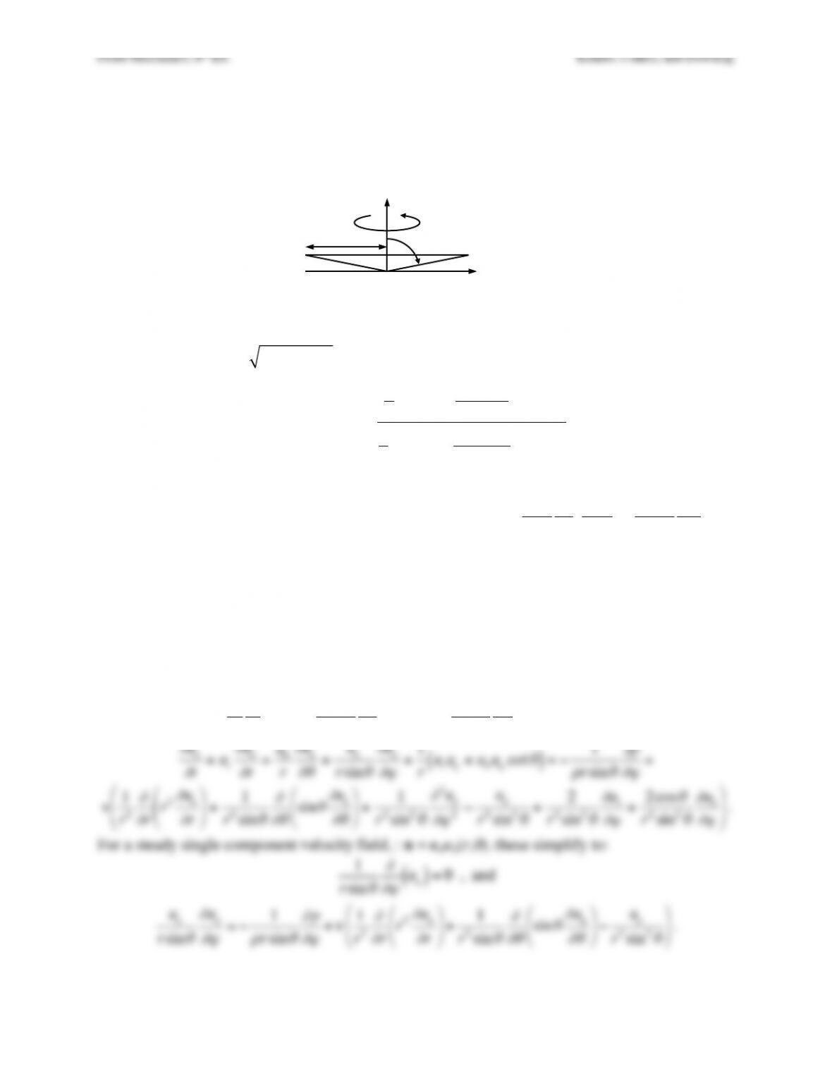
Exercise 9.49. Consider the geometry of a cone and plate rheometer. A flat cone with radius R
and apex angle of
θ
1, slightly less than
π
/2, touches a large stationary horizontal flat plate at the
origin and rotates at a constant rate Ω about the vertical z-axis. A viscous fluid with density
ρ
and viscosity
µ
fills the gap between the cone and the plate.
a) Assuming the fluid’s velocity is steady with a single component: u = e
ϕ
u
ϕ
(r,
θ
), use the
continuity equation and the azimuthal momentum equation for creeping flow in spherical
coordinates, where
r=x2+y2+z2
, to find:
u
ϕ
(r,
θ
)=Ωrsin
θ
1
1
2sin
θ
⋅ln 1+cos
θ
1 – cos
θ
#
$
%&
‘
(+cot
θ
1
2sin
θ
1⋅ln 1+cos
θ
1
1 – cos
θ
1
#
$
%&
‘
(+cot
θ
1
)
*
+
+
+
+
,
–
.
.
.
.
.
The boundary conditions here are u
ϕ
(r,
π
/2) = 0, and u
ϕ
(r,
θ
1) = rΩsin
θ
1.
b) Use this to determine the polar-azimuthal shear stress:
τθϕ
=
µ
sin
θ
r
∂
∂θ
u
ϕ
sin
θ
&
‘
(
)
*
+ +1
rsin
θ
∂
u
θ
∂φ
–
.
/
0
1
2
.
c) Simplify the velocity field and shear stress results when
θ
and
θ
1 both approach π/2.
d) A torque of 3.0 N-m causes the cone to rotate with an angular velocity of 1.5 rad/s. If the
radius of the cone is R = 6.35 cm and 90° –
θ
1 = 0.30°, what is the viscosity of the fluid?
e) For the conditions in part d) with
ρ
= 103 kg/m3, compare
ρ
Ω2R2 to
τθϕ
. Is neglect of fluid
inertia justified here?
Solution 9.49. a) The continuity and azimuthal momentum equation in spherical coordinates are:
1
r2
∂
∂
r
r2ur
( )
+1
rsin
θ
∂
∂θ
u
θ
sin
θ
( )
+1
rsin
θ
∂
∂ϕ
u
ϕ
( )
=0
, and
∂
u
ϕ
∂
t+ur
∂
u
ϕ
∂
r+u
θ
r
∂
u
ϕ
∂θ
+u
ϕ
rsin
θ
∂
u
ϕ
∂ϕ
+1
ruru
ϕ
+u
θ
u
ϕ
cot
θ
( )
=−1
ρ
rsin
θ
∂
p
∂ϕ
+
ν
1
r2
∂
∂
r
r2
∂
u
ϕ
∂
r
%
&
‘
(
)
* +1
r2sin
θ
∂
∂θ
sin
θ∂
u
ϕ
∂θ
%
&
‘
(
)
* +1
r2sin2
θ
∂
2u
ϕ
∂ϕ
2−u
ϕ
r2sin2
θ
+2
r2sin2
θ
∂
ur
∂ϕ
+2cos
θ
r2sin2
θ
∂
u
θ
∂ϕ
%
&
‘
(
)
*
.
For a steady single component velocity field, : u = e
ϕ
u
ϕ
(r,
θ
), these simplify to:
1
rsin
θ
∂
∂ϕ
u
ϕ
( )
=0
, and
u
ϕ
rsin
θ
∂
u
ϕ
∂ϕ
=−1
ρ
rsin
θ
∂
p
∂ϕ
+
ν
1
r2
∂
∂
rr2
∂
u
ϕ
∂
r
“
#
$%
&
‘+1
r2sin
θ
∂
∂θ
sin
θ∂
u
ϕ
∂θ
“
#
$%
&
‘−u
ϕ
r2sin2
θ
“
#
$%
&
‘
.
θ
1!
R!
z!
x or y!
Ω”
Fluid Mechanics, 6th Ed. Kundu, Cohen, and Dowling
The reduced continuity equation is satisfied identically by form of the given solution. The
momentum equation can be simplified to creeping flow by dropping the term on the left. In
addition, since velocity field is independent of
ϕ
, assume that the pressure field is similarly
independent of
ϕ
so the first term on the right of the reduced azimuthal momentum equation is
also zero. This leaves:
Fluid Mechanics, 6th Ed. Kundu, Cohen, and Dowling
b) The approach here is to take the part a) velocity field and plug it into the shear stress formula.
To simplify the effort set
C(
θ
1)=Ωsin
θ
1
sin
θ
1
2ln 1+cos
θ
1
1−cos
θ
1
%
&
‘
(
)
* +cot
θ
1
%
&
‘
(
)
*
, so that
u
ϕ
(r,
θ
)=rC(
θ
1)sin
θ
2ln 1+cos
θ
1−cos
θ
%
&
‘ (
)
* +cot
θ
%
&
‘
(
)
*
. Continue to the differentiations:
∂
u
ϕ∂ϕ
=0
, and
∂
∂θ
u
ϕ
sin
θ
%
&
‘
(
)
* =rC(
θ
1)
∂
∂θ
1
2ln 1+cos
θ
( )
−1
2ln 1−cos
θ
( )
+cos
θ
sin2
θ
%
&
‘ (
)
*
∂
∂θ
u
ϕ
sin
θ
%
&
‘
(
)
* =rC(
θ
1)−sin
θ
2(1+cos
θ
)−sin
θ
2(1−cos
θ
)−sin
θ
sin2
θ
−2cos2
θ
sin3
θ
%
&
‘
(
)
*
sin
θ
r
∂
∂θ
u
ϕ
sin
θ
%
&
‘
(
)
* =C(
θ
1)−sin2
θ
2(1+cos
θ
)−sin2
θ
2(1−cos
θ
)−1−2cos2
θ
sin2
θ
%
&
‘
(
)
*
Use some trigonometric identities for simplification.
sin
θ
r
∂
∂θ
u
ϕ
sin
θ
%
&
‘
(
)
* =C(
θ
1)−(1−cos
θ
)
2−1+cos
θ
2−1−2cos2
θ
sin2
θ
%
&
‘
(
)
* =−2C(
θ
1) 1+cos2
θ
sin2
θ
%
&
‘
(
)
* =−2C(
θ
1)
sin2
θ
Thus,
τθϕ
=
µ
sin
θ
r
∂
∂θ
u
ϕ
sin
θ
&
‘
(
)
*
+ +1
rsin
θ
∂
u
θ
∂φ
–
.
/
0
1
2 =−
µ
2C(
θ
1)
sin2
θ
, which does not depend on r!
c) As
θ
→ π/2, cos(
θ
) → π/2 –
θ
, and sin(
θ
) → 1, thus
C(
θ
1)≅ Ω 1
2ln 1+
π
/2 −
θ
1
1−
π
/2 +
θ
1
‘
(
)
*
+
, +
π
/2 −
θ
1
1
‘
(
)
*
+
, ≅ Ω 2
π
/2 −
θ
1
( )
[ ]
,
u
ϕ
(r,
θ
)≅2rC(
θ
1)
π
/2 −
θ
( )
=Ωr
π
/2 −
θ
π
/2 −
θ
1
(
)
*
+
,
–
, and
τθϕ
=−
µ
Ω
π
/2 −
θ
1
d) The torque necessary to turn the cone will be:
M=−
τ
r2d
θ
d
r=0
R
∫r=2
πτ
R33=2
πµ
ΩR3
3(
π
/2 −
θ
1)
.
Solve this for the viscosity and evaluate:
µ
=3(
π
/ 2 −
θ
1)M
2
π
ΩR3=3(0.30°
π
/180°)(3.0Nm)
2
π
(1.50rad /s)(0.0635m)3
= 19.5 kgm-1s-1
e) Here:
ρ
Ω2R2=
(103kg/m3)(1.50rad/s)2(0.0635m)2 = 9.07 Pa, while