Fluid Mechanics, 6th Ed. Kundu, Cohen, and Dowling
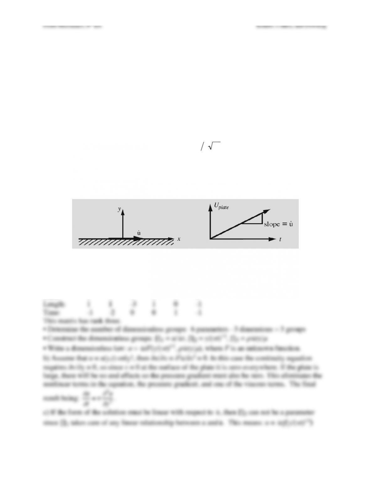
Exercise 9.31. A large flat plate below an infinite stationary incompressible viscous fluid is set
in motion with a constant acceleration,
˙
u
, at t = 0. A prediction for the subsequent fluid motion,
u(y,t), is sought.
a) Use dimensional analysis to write a physical law for u(y,t) in this flow.
b) Starting from the x-component of (8.1) determine a linear partial differential equation for
u(y,t).
c) The linearity of the equation obtained for part c) suggests that u(y,t) must be directly
proportional to
˙
u
. Simplify your dimensional analysis to incorporate this requirement.
d) Let
η
= y/(
ν
t)1/2 be the independent variable, and derive a second-order ordinary linear
differential equation for the unknown function f(
η
) left from the dimensional analysis.
e) From an analogy between fluid acceleration in this problem and fluid velocity in Stokes’ first
problem, deduce the solution
u(y,t)=˙
u 1−erf y2
ν
$
t
( )
[ ]
d$
t
0
t
∫
and show that it solves the
equation of part b).
f) Determine f(
η
) and – if your patience holds out – show that it solves the equation found in part
d).
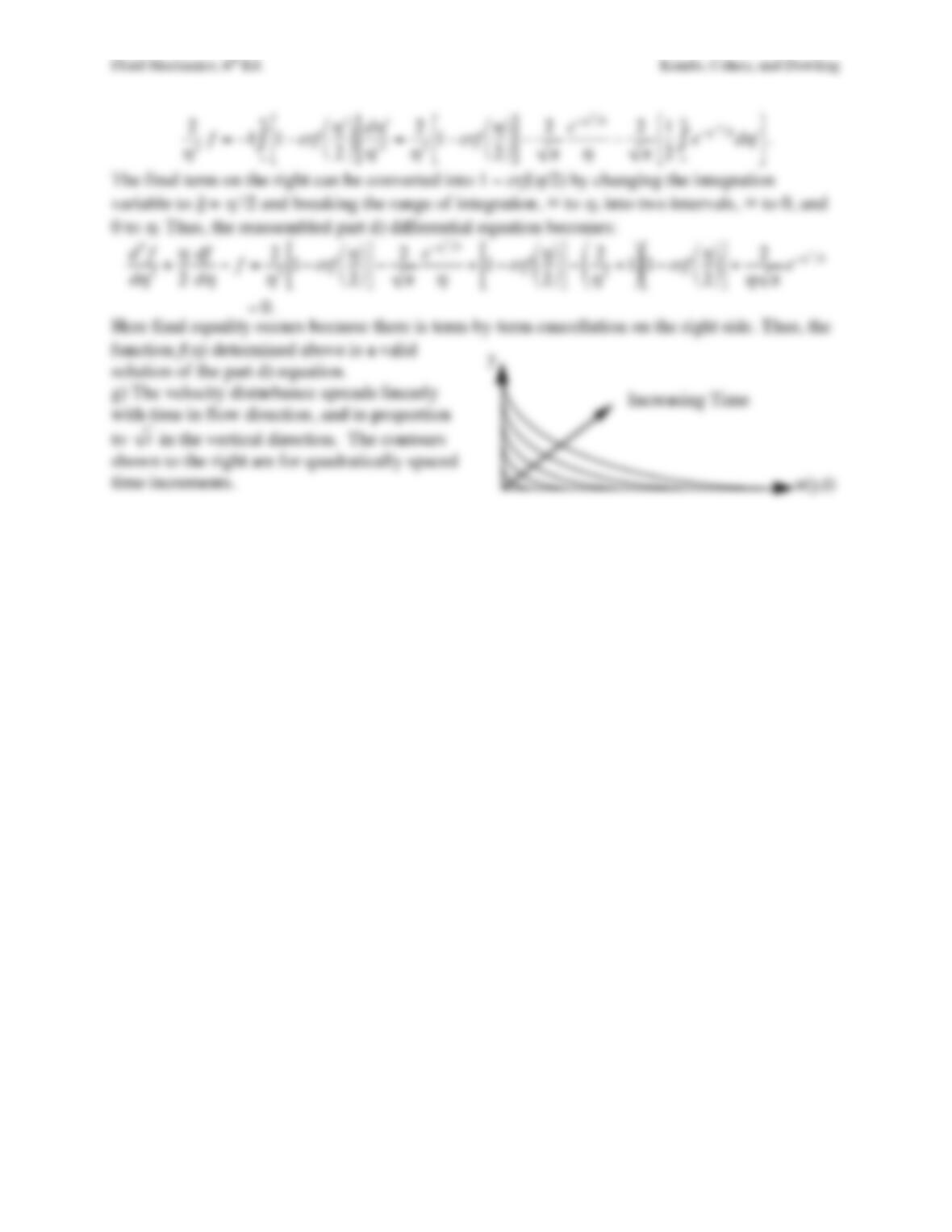
g) Sketch the expected velocity profile shapes for several different times. Note the direction of
increasing time on your sketch.
Solution 9.31. a) The problem parameters are:
˙
u
,
ρ
, y, t, and
µ
. The solution parameter is u.
• Create the parameter matrix:
u
˙
u
ρ
y t
µ
––––––––––––––––––––––––––––––––––
Mass: 0 0 1 0 0 1
Length: 1 1 -3 1 0 -1
˙
u
˙
u
˙
u
˙
u
˙
u
Fluid Mechanics, 6th Ed. Kundu, Cohen, and Dowling
d) First convert derivatives, then differentiate being sure to account for the pre-factor of
˙
u
t.
∂
∂
t=
∂η
∂
t
∂
∂η
=−1
2
y
ν
t3
∂
∂η
=−
η
2t
∂
∂η
, and
∂
∂
y=
∂η
∂
y
∂
∂η
=1
ν
t
∂
∂η
.
Therefore:
∂
u
∂
t=
∂
∂
t˙
u tf (
η
)
[ ]
=˙
u f−˙
u t
η
2t
df
d
η
, and
ν∂
2u
∂
y2=
∂
2
∂
y2˙
u tf (
η
)
[ ]
=
ν
˙
u t1
ν
t
d2f
d
η
2
.
˙
u
Fluid Mechanics, 6th Ed. Kundu, Cohen, and Dowling
Set
“
η
=y
ν
“
t
so that
d“
η
=−y2
ν
“
t 3
( )
d“
t =−
ν
2y2
( )
“
η
3d“
t
and
d“
t =−2y2
ν
“
η
3
( )
d“
η
, and use
this in the equation for u(y, t):
u(y,t)=˙
u 1−2
π
exp(−
ξ
2)d
ξ
0
η
‘ 2
∫
‘
(
)
*
+
,
∞
η
∫−2y2
ν
/
η
3
0
1
2
3
4
5
d/
η
.
Multiply by t outside the integral, divide by t inside the integral, and recognize the definition of
Fluid Mechanics, 6th Ed. Kundu, Cohen, and Dowling
Fluid Mechanics, 6th Ed. Kundu, Cohen, and Dowling
Exercise 9.32. a) When z is complex, the small-argument expansion of the zeroth-order Bessel
function
Jo(z)=1−1
4z2+…
remains valid. Use this to show that (9.43) reduces to (9.6) as
ω
→0
when dp/dz = Δp/L. The next term in the series is
1
64 z4
. At what value of
a
ν ω
is the
magnitude of this term equal to 5% of the second term.
b) When z is complex, the large-argument expansion of the zeroth-order Bessel function
Jo(z)≅2
π
z
( )
1 2 cos z−1
4
π
#
$%
&
remains valid for |arg(z)| <
π
. Use this to show that (9.43) reduces to
the velocity profile of a viscous boundary layer on a plane wall beneath an oscillating flow as
ω
→ ∞
:
uz(y,t)=−Δp
ρω
Lsin(
ω
t)−exp −y
ω
2
ν
#
$
%
&
‘
(sin
ω
t−y
ω
2
ν
)
*
+,
–
.
/
0
1
1
2
3
4
4
,
where y is the distance from the tube wall, R = a – y, y << a, and dp/dz = Δp/L.
Solution 9.32. a) Start from (9.43):
uz(R,t)=Re iΔp
ωρ
L1−Jo
i3 2 R
ν ω
#
$
%
%
&
‘
(
(Jo
i3 2a
ν ω
#
$
%
%
&
‘
(
(
)
*
+
+
,
–
.
.ei
ω
t
/
0
1
2
1
3
4
1
5
1
, and
use the small argument form of Jo for the limit
ω
→0
:
lim
ω
→0uz(R,t)=lim
ω
→0
Re iΔp
ωρ
L1−
1−1
4
i3 2 R
ν ω
$
%
&
&
‘
(
)
)
+…
1−1
4
i3 2a
ν ω
$
%
&
&
‘
(
)
)
2
+…
*
+
,
,
,
,
,
–
.
/
/
/
/
/
ei
ω
t
1
2
2
3
2
2
5
2
2
6
2
2
=lim
ω
→0
Re iΔp
ωρ
L1−
1+i
ω
R2
4
ν
+…
1+i
ω
a2
4
ν
+…
*
+
,
,
,
,
–
.
/
/
/
/
ei
ω
t
0
1
2
2
3
2
2
4
5
2
2
6
2
2
.
Continue simplifying:
lim
ω
→0
uz(R,t)=lim
ω
→0
Re iΔp
ωρ
L1−1+i
ω
R2
4
ν
−i
ω
a2
4
ν
+…
$
%
&‘
(
)
*
+
,–
.
/ei
ω
t
0
1
2
3
2
4
5
2
6
2
=lim
ω
→0
Re iΔp
ωρ
L−i
ω
R2
4
ν
+i
ω
a2
4
ν
*
+
,–
.
/ei
ω
t
0
1
3
4
5
6
=Re Δp
ρ
L+R2
4
ν
−a2
4
ν
*
+
,–
.
/
0
1
3
4
5
6
=1
4
µ
−Δp
L
$
%
&‘
(
)a2−R2
( )
and this is the same as (9.6) when the pressure gradient is Δp/L.
To determine when
1
64 z4
is 5% of
1
4z2
, set
(0.05) 1
z2=1
z4
and determine z. The
Fluid Mechanics, 6th Ed. Kundu, Cohen, and Dowling
cos z−
π
4
“
#
$%
&
‘=1
2exp i−1
2+i
2
“
#
$%
&
‘R
ν ω
−i
π
4
(
)
*
+
*
,
–
*
.
*+exp −i−1
2+i
2
“
#
$%
&
‘R
ν ω
+i
π
4
(
)
*
+
*
,
–
*
.
*
/
0
1
1
2
3
4
4
=1
2exp −i
2−1
2
“
#
$%
&
‘R
ν ω
−i
π
4
(
)
*
+
*
,
–
*
.
*+exp i
2+1
2
“
#
$%
&
‘R
ν ω
+i
π
4
(
)
*
+
*
,
–
*
.
*
/
0
1
1
2
3
4
4
When
ω
→ ∞
, the first term becomes exponentially small, so
ω
→ ∞
ω
→ ∞
ω
→ ∞
So, in this limit:
Jo
i3 2 R
ν ω
!
“
#
#
$
%
&
&
Jo
i3 2a
ν ω
!
“
#
#
$
%
&
&
=
2
π
ν ω
i3 2 (a−y)
ei
π
4
2exp a(1+i)
2
ν ω
!
“
#
#
$
%
&
&exp −(1+i)
2
ν ω
y
!
“
#
#
$
%
&
&
2
π
ν ω
i3 2a
ei
π
4
2exp a(1+i)
2
ν ω
!
“
#
#
$
%
&
&
=a
a−yexp −(1+i)
2
ν ω
y
!
“
#
#
$
%
&
&
≅exp −(1+i)
2
ν ω
y
!
“
#
#
$
%
&
&
where the final approximate equality holds when y << a. Now substitute this approximate ratio
of Bessel functions into (9.43) to find:
uz(y,t)=Re iΔp
ωρ
L1−exp −(1+i)y
2
ν ω
#
$
%
%
&
‘
(
(
)
*
+
+
,
–
.
.ei
ω
t
/
0
1
2
1
3
4
1
5
1
=Re iΔp
ωρ
Lei
ω
t−exp −y
2
ν ω
#
$
%
%
&
‘
(
(exp i
ω
t−iy
2
ν ω
#
$
%
%
&
‘
(
(
)
*
+
+
,
–
.
.
/
0
1
2
1
3
4
1
5
1
.
Take the real part to reach:
uz(y,t)=−Δp
ωρ
Lsin(
ω
t)−exp −y
2
ν ω
#
$
%
%
&
‘
(
(sin
ω
t−y
2
ν ω
#
$
%
%
&
‘
(
(
)
*
+
+
,
–
.
.
,
and this is the desired result.
Fluid Mechanics, 6th Ed. Kundu, Cohen, and Dowling
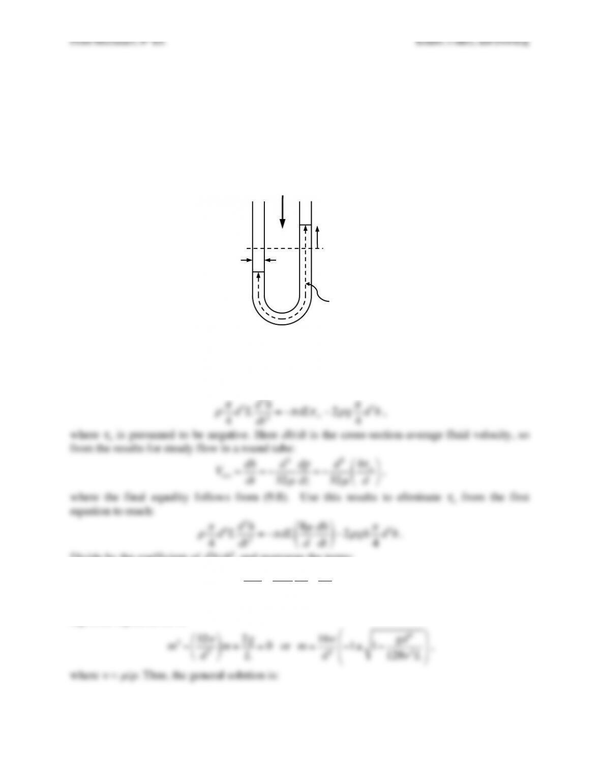
Exercise 9.33. A round tube bent into a U-shape having inner diameter d holds a column of
liquid with overall length L. Initially the column of liquid is pushed upward on the right side of
the U-tube and downward on the left side of the U-tube so that the two liquid surfaces are a
vertical distance 2ho apart. If the liquid has density
ρ
and viscosity
µ
, and the column is released
from rest, find and solve an approximate ordinary differential equation that describes the
subsequent damped oscillations of h(t), the liquid height above equilibrium in the right side of
the U-tube, assuming that the flow profile at any time throughout the tube is parabolic. Under
what condition(s) is this approximate solution valid? Will oscillations occur in this parameter
regime?
Solution 9.33. This is the fluid mechanical pendulum with viscous effects included. Use
Newton’s second law for the mass of fluid in the water column. The unbalanced gravitational
force tends to decrease h(t) and is –2
ρ
gh(
π
d2/4) and the wall shear stress opposes the motion.
Thus:
ρπ
4d2Ld2h
dt2=−
π
dL
τ
w−2
ρ
g
π
4d2h
,
where
τ
w is presumed to be negative. Here dh/dt is the cross-section-average fluid velocity, so
from the results for steady flow in a round tube:
Vave =dh
dt =−d2
32
µ
dp
dz =−d2
32
µ
4
τ
w
d
“
#
$%
&
‘
,
where the final equality follows from (9.8). Use this results to eliminate
τ
w from the first
equation to reach:
ρπ
4d2Ld2h
dt2=−
π
dL 8
µ
d
dh
dt
“
#
$%
&
‘−2
ρ
gh
π
4d2h
.
Divide by the coefficient of d2h/dt2, and rearrange the terms:
d2h
dt2+32
µ
ρ
d2
dh
dt +2g
Lh=0
. ($)
This equation can be solved by assuming an exponential solution: h(t) = hoe–mt, which leads to an
algebraic equation for m:
m2−32
ν
d2
“
#
$%
&
‘m+2g
L=0
or
m=16
ν
d2−1±1−gd4
128
ν
2L
“
#
$
$
%
&
‘
‘
,
where
ν
=
µ
/
ρ
. Thus, the general solution is:
L!
d!
h(t)!
g!
Fluid Mechanics, 6th Ed. Kundu, Cohen, and Dowling
h(t)=A+exp 16
ν
t
d2−1+1−gd4
128
ν
2L
“
#
$
$
%
&
‘
‘
(
)
*
+
*
,
–
*
.
*
+A−exp 16
ν
t
d2−1−1−gd4
128
ν
2L
“
#
$
$
%
&
‘
‘
(
)
*
+
*
,
–
*
.
*
.
The constants can be determined from the initial conditions, h(0) = ho, and dh/dt = 0,
which lead to two algebraic equations:
ho=A++A−
, and
0=A+
16
ν
d2−1+1−gd4
128
ν
2L
“
#
$
$
%
&
‘
‘+A−
16
ν
d2−1−1−gd4
128
ν
2L
“
#
$
$
%
&
‘
‘
.
Thus, the constants are:
A+=ho
2
1+1
1−
ψ
“
#
$
$
%
&
‘
‘
, and
A−=ho
2
1−1
1−
ψ
“
#
$
$
%
&
‘
‘
,
where
ψ
= gd4/128
ν
2L. The final solution is:
h(t)=ho
21+1
1−
ψ
“
#
$
$
%
&
‘
‘exp 16
ν
t
d2−1+1−
ψ
( )
(
)
*
+
,
–+ho
21−1
1−
ψ
“
#
$
$
%
&
‘
‘exp 16
ν
t
d2−1−1−
ψ
( )
(
)
*
+
,
–
. (&)
This approximate solution will be valid when d << L so the nearly the entire water
This solution can be obtained directly from ($) by dropping the acceleration term and solving.
Fluid Mechanics, 6th Ed. Kundu, Cohen, and Dowling
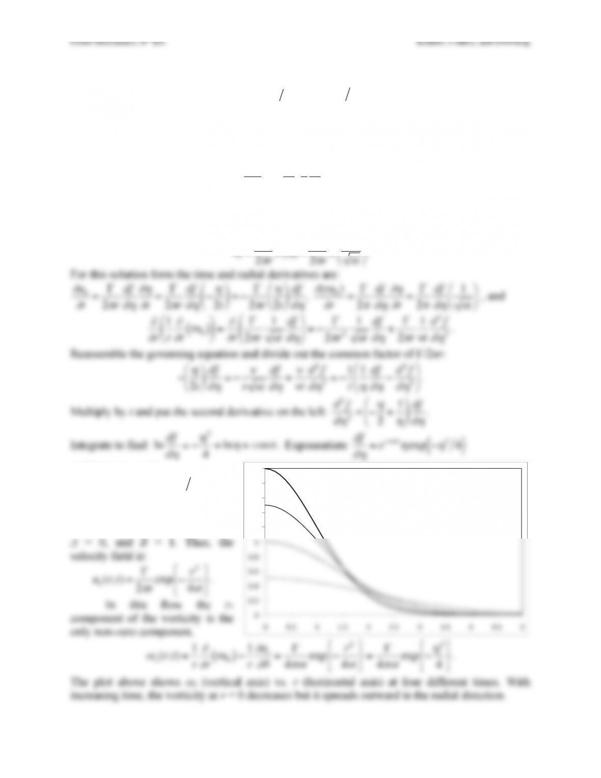
Exercise 9.34. Suppose a line vortex of circulation Γ is suddenly introduced into a fluid at rest at
t = 0. Show that the solution is
u
θ
(r,t)=Γ2
π
r
( )
exp −r24
ν
t
{ }
. Sketch the velocity distribution
at different times. Calculate and plot the vorticity, and observe how it diffuses outward.
Solution 9.34. The solution to this problem is very similar to the decay of a line vortex (see
Example 9.8). In two-dimensional (r,
θ
)-polar coordinates, the governing equation is:
∂
u
θ
∂
t=
ν∂
∂
r
1
r
∂
∂
r
ru
θ
( )
%
&
‘ (
)
*
+
,
–
.
/
0
.
The boundary conditions on the velocity u
θ
(r, t) are
u
θ
(r,0+) = 0, u
θ
(r,∞) = Γ/2πr, and u
θ
(∞, t) = 0.
In this case the second boundary condition suggests a similarity solution of the form:
u
θ
=Γ
2
π
rf
η
( )
=Γ
2
π
rfr
ν
t
‘
(
) *
+
,
.
For this solution form the time and radial derivatives are:
and integrate again:
f=A+Bexp −
η
24
{ }
.
The constants A and B can be
determined from the boundary
conditions: f(0) = 1, and f(∞) = 1;
A = 0, and B = 1. Thus, the
increasing time, the vorticity ar r = 0 decreases but it spreads outward in the radial direction.
(“
(#$”
(#%”
(#&”
(#'”
$”
Fluid Mechanics, 6th Ed. Kundu, Cohen, and Dowling
Exercise 9.35. Following Taylor and Green (1937), consider the two-dimensional vortex flow
field with constant density
ρ
:
u=(u,v)=Asin(kx)cos(ky), Bcos(kx)sin(ky)
( )
.
a) If the flow is steady and inviscid, and A and B are constants, explicitly determine the pressure,
p(x,y), in terms of x, y, A,
ρ
, and k from (4.10) and (9.1) in two dimensions.
b) If the flow field is unsteady and viscous (with viscosity
µ
), A and B are functions of time t,
and A = Ao at t = 0, determine A(t), B(t), and p(x,y,t) so that the given u is an exact solution of
(4.10) and (9.1) in two dimensions.
c) How long does it take for A(t) to fall to Ao/2? Does the parametric dependence of this decay
time follow typical diffusion scaling?
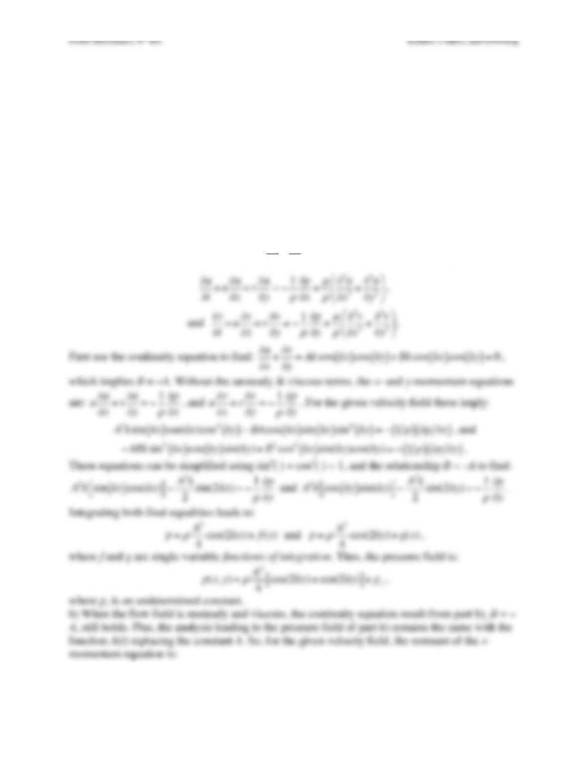
Solution 9.35. a) Here
ρ
= const. so (4.10) and (9.1) simplify to:
∂u
∂x+∂v
∂y=0
,
∂u
∂t+u∂u
∂x+v∂u
∂y=−1
ρ
∂p
∂x+
µ
ρ
∂2u
∂x2+∂2u
∂y2
#
$
%&
‘
(
,
and
∂v
∂t+u∂v
∂x+v∂v
∂y=−1
ρ
∂p
∂y+
µ
ρ
∂2v
∂x2+∂2v
∂y2
#
$
%&
‘
(
.
First use the continuity equation to find:
∂u
∂x+∂v
∂y=Ak cos kx
( )
cos ky
( )
+Bk cos kx
( )
cos ky
( )
=0
,
which implies B = –A. Without the unsteady & viscous terms, the x– and y-momentum equations
are:
u∂u
∂x+v∂u
∂y=−1
ρ
∂p
∂x
, and
u∂v
∂x+v∂v
∂y=−1
ρ
∂p
∂y
. For the given velocity field these imply:
A2ksin kx
( )
cos(kx)cos2ky
( )
−BA cos kx
( )
sin kx
( )
sin2ky
( )
=−1
ρ
( )
∂p∂x
( )
, and
−ABk sin2kx
( )
cos ky
( )
sin(ky)+B2cos2kx
( )
sin(ky)cos(ky)=−1
ρ
( )
∂p∂y
( )
.
These equations can be simplified using sin2( ) + cos2( ) = 1, and the relationship B = –A to find:
A2ksin kx
( )
cos(kx)
!
“#
$=A2k
2sin(2kx)=−1
ρ
∂p
∂x
and
A2kcos ky
( )
sin(ky)
!
“#
$=A2k
2sin(2ky)=−1
ρ
∂p
∂y
.
Integrating both final equalities leads to:
p=
ρ
A2
4cos(2kx)+f(y)
and
p=
ρ
A2
4cos(2ky)+g(x)
,
where f and g are single-variable functions of integration. Thus, the pressure field is:
p(x,y)=
ρ
A2
4cos(2kx)+cos(2ky)
[ ]
+po
,
where po is an undetermined constant.
b) When the flow field is unsteady and viscous, the continuity equation result from part b), B = –
A, still holds. Plus, the analysis leading to the pressure field of part b) remains the same with the
function A(t) replacing the constant A. So, for the given velocity field, the remnant of the x–
momentum equation is:
Fluid Mechanics, 6th Ed. Kundu, Cohen, and Dowling
Fluid Mechanics, 6th Ed. Kundu, Cohen, and Dowling
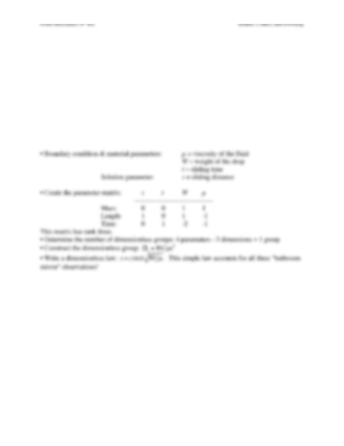
Exercise 9.36. Obtain several liquids of differing viscosity (water, cooking oil, pancake syrup,
shampoo, etc.). Using an eyedropper, a small spoon, or your finger, place a drop of each on a
smooth vertical surface (a bathroom mirror perhaps) and measure how far the drops have moved
or extended in a known period of time (perhaps a minute or two). Try to make the mass of all the
drops equal. Using dimensional analysis, determine how the drop-sliding distance depends on the
other parameters. Does this match your experimental results?
Solution 9.36. The experiments yield the following three qualitative results. 1) The drops of the
more viscous liquids do not slide as quickly as those of the less viscous liquids. 2) The drops
slow down as time increases. 3) Bigger drops go farther. Water does not behave like oils or
liquid soaps because its surface tension is large enough to influence the motion of the sliding
drop. Here, we wish to use the simplest possible dimensional analysis so surface tension will be
ignored.
• Boundary condition & material parameters: µ = viscosity of the fluid
Fluid Mechanics, 6th Ed. Kundu, Cohen, and Dowling
Exercise 9.37. A drop of an incompressible viscous liquid is allowed to spread on a flat
horizontal surface under the action of gravity. Assume the drop spreads in an axisymmetric
fashion and use cylindrical coordinates (R,
ϕ
, z). Ignore the effects of surface tension.
a) Show that conservation of mass implies:
∂
h
∂
t+1
R
∂
∂
R
R udz
o
h
∫
( )
=0
, where u = u(R,z,t) is the
horizontal velocity within the drop, and h = h(R,t) is the thickness of the spreading drop.
b) Assume that the lubrication approximation applies to the horizontal velocity profile, i.e.
u(R,z,t)=a(R,t)+b(R,t)z+c(R,t)z2
, apply the appropriate boundary conditions on the upper
and lower drop surfaces, and require a pressure & shear-stress force balance within a differential
control volume h(R,t)RdRd
θ
to show that:
u(R,z,t)=−g
2
ν
∂
h
∂
Rz(2h−z)
.
c) Combine the results of a) and b) to find
∂
h
∂
t=g
3
ν
R
∂
∂
RRh3
∂
h
∂
R
$
%
& ‘
(
)
.
d) Assume a similarity solution:
h(R,t)=A
tnf(
η
)
with
η
=BR
tm
, use the result of part c) and
2
π
h(R,t)RdR =V
o
Rmax (t)
∫
where Rmax(t) is the radius of the spreading drop and V is the initial
volume of the drop to determine m = 1/8, n = 1/4, and a single nonlinear ordinary differential
equation for f(
η
) involving only A, B, g/
ν
, and
η
. You need not solve this equation for f. [Given
that
f→0
as
η
→ ∞
, there will be a finite value of
η
for which f is effectively zero. If this
value of
η
is
η
max then the radius of the spreading drop, R(t), will be:
Rmax (t)=
η
max tmB
.]
Solution 9.37. a) Consider a stationary “ring” control volume that has inner radius of R, outer
radius of R + dR, and height h(R,t). There is no flow out through the underside of the CV, but all
three other sides contribute a term to the mass balance.
−2
π
R udz
0
h(R,t)
∫+2
π
(R+dR)udz
0
h(R+dR ,t)
∫+2
π
(R+dR /2)
∂
h
∂
t
dR =0
Fluid Mechanics, 6th Ed. Kundu, Cohen, and Dowling
p(R)
0
h(R,t)
∫Rd
θ
dz −p(R+dR)
0
h(R+dR,t)
∫(R+dR)d
θ
dz −
τ
wRdRd
θ
=0
Here take atmospheric pressure as the zero or reference pressure level. The pressure that matters
will be hydrostatic,
p(R,t)=
ρ
g h(R,t)−z
( )
so that the above equation becomes:
ρ
gh2(R,t)
2Rd
θ
−
ρ
gh2(R+dR,t)
2(R+dR)d
θ
−
τ
wRdRd
θ
=0
.
Divide this by Rd
θ
, drop the higher order term, and rearrange to form the definition of a
derivative:
−1
dR
ρ
gh2(R+dR,t)
2−
ρ
gh2(R,t)
2
$
%
&
‘
(
) =
τ
w
Take the limit as
dR →0
and perform the radial derivative:
τ
w=−
∂
∂
R
ρ
gh2
2
&
‘
(
)
*
+ =−
ρ
gh
∂
h
∂
R
.
Place
ν
=
µρ
and this wall-shear-stress-static-pressure-gradient relationship into the velocity
profile formula to simplify it and eliminate
τ
w:
u(R,z,t)=−g
2
ν
∂
h
∂
Rz(2h−z)
.
c) Use the result of part b) and perform the integration specified in the result of part a)
udz
o
h
∫=−g
2
ν
∂
h
∂
Rz(2h−z)dz
o
h
∫=−g
2
ν
∂
h
∂
R2hz2
2−z3
3
&
‘
(
)
*
+
0
h
=−gh3
3
ν
∂
h
∂
R
Put this into the result of part a) and bring the constants outside the radial differentiation to find:
∂
h
∂
t−g
3
ν
R
∂
∂
RRh3
∂
h
∂
R
%
&
‘ (
)
* =0
.
d) First consider a CV that entirely encloses the drop and moves with it. Thus, conservation of
mass in this case implies:
d
dt 2
π
h(R,t)RdR
0
Rmax (t)
∫
( )
=0
because there are no fluxes crossing the
CV boundary. Integrate once in time to find:
2
π
h(R,t)RdR =const
0
Rmax (t)
∫
. The constant can be
evaluated as V, the volume of the drop, at the initial time (or any other time); thus,
2
π
h(R,t)RdR =V
0
Rmax (t)
∫
.
Now use the proposed similarity solution form,
h(R,t)=A
tnf(
η
)
with
η
=BR
tm
, and perform the
various differentiations:
∂
∂
th(R,t)=−nA
tn+1f(
η
)+A
tn%
f (
η
)−mBR
tm+1
&
‘
( )
*
+ =−nA
tn+1f(
η
)−mA
tn+1
η
%
f (
η
)
,
∂
∂
Rh(R,t)=A
tn#
f (
η
)B
tm=AB
tn+m#
f (
η
)
,
Rh3
∂
∂
rh(R,t)=RA4B
t4n+mf3(
η
)$
f (
η
)
, so
1
R
∂
∂
RRh3
∂
∂
Rh(R,t)
#
$
% &
‘
( =A4B
Rt4n+mf3(
η
)*
f (
η
)+A4B2
t4n+2m3f2(
η
)*
f (
η
)+f3(
η
)* *
f (
η
)
( )
=A4B2
t4n+2m
η
f3(
η
)#
f (
η
)+A4B2
t4n+2m3f2(
η
)#
f (
η
)+f3(
η
)# #
f (
η
)
( )
.
Thus, the field equation determined for part c) implies:
Fluid Mechanics, 6th Ed. Kundu, Cohen, and Dowling
Fluid Mechanics, 6th Ed. Kundu, Cohen, and Dowling
Exercise 9.38. Obtain a clean flat glass plate, a watch, a ruler, and some non-volatile oil that is
more viscous than water. The plate and oil should be at room temperature. Dip the tip of one of
your fingers in the oil and smear it over the center of the plate so that a thin bubble-free oil film
covers a circular area ~10 to 15 cm in diameter. Set the plate on a horizontal surface and place a
single drop of oil at the center of the oil-film area and observe how the drop spreads. Measure
the spreading drop’s diameter 1, 10, 102, 103, and 104 seconds after the drop is placed on the
plate. Plot your results and determine if the spreading drop diameter grows as t1/8 (the predicted
drop-diameter time dependence from the prior exercise) to within experimental error.
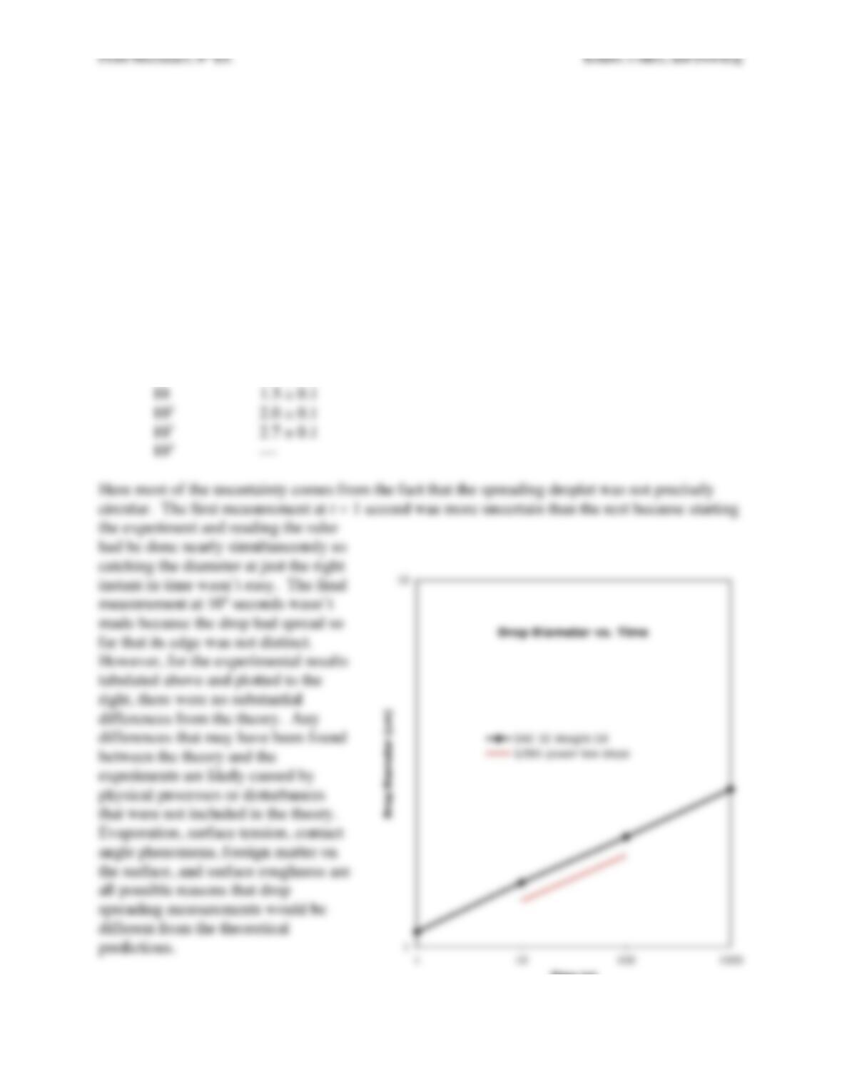
Solution 9.38. For this kitchen-or-garage experiment, the third author of this textbook used the
glass plate from the front of a document frame and SAE 30-Weight motor oil to obtain the
following measurements.
time (s) Drop Diameter (cm)
1 1.1 ± 0.2
10 1.5 ± 0.1
Fluid Mechanics, 6th Ed. Kundu, Cohen, and Dowling
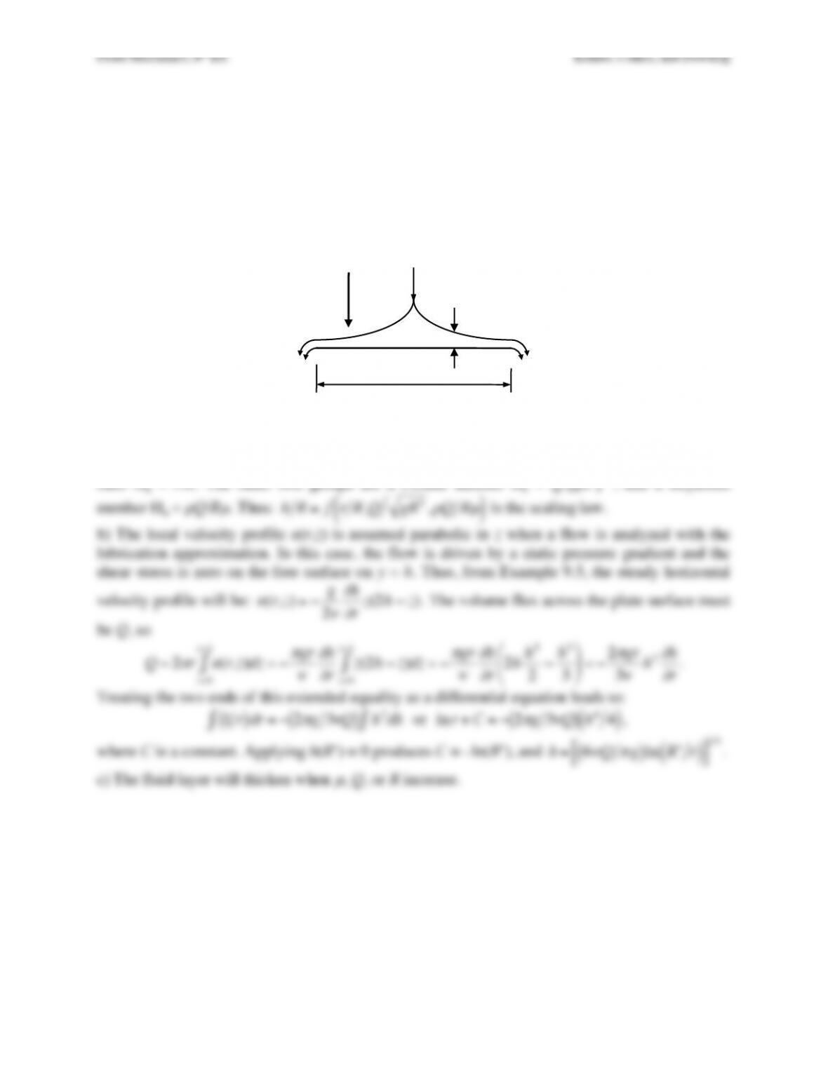
Exercise 9.39. A fine stream of a viscous fluid with density
ρ
and viscosity
µ
falls slowly at a
constant volume flow rate Q onto the center of a flat horizontal circular disk of radius R. The
fluid flows steadily under the action of gravity g from the center of the disk to its edge in a layer
of thickness h(r), where r is the radial coordinate. For the following items, assume Q is constant,
and apply the approximate boundary condition h(R+) = 0, where R+ is a radial location just
beyond the edge of the disk.
a) Determine a scaling law for h from dimensional analysis.
b) Using the lubrication approximation determine a formula for h(r) that is valid for 0 < r < R.
c) Increasing which parameters increases the thickness of the fluid layer on the disk.
Solution 9.39. a) There are six parameters (h, r, Q, g, R,
ρ
, and
µ
) and all three fundamental
dimensions are present so there will be 7 – 3 = 4 dimensionless parameters. Here h is the solution
parameter so put it in the first group, Π1 = h/R. The second group is also a simple length scale
ratio Π2 = r/R. The other two groups are a Froude number Π3 = Q/[gR5]1/2, and a Reynolds
number Π4 =
ρ
Q/R
µ
. Thus:
h R =f r R,Q gR5,
ρ
Q R
µ
( )
is the scaling law.
h(r)!
2R!
g!Q!
Fluid Mechanics, 6th Ed. Kundu, Cohen, and Dowling
Exercise 9.40. An infinite flat plate located at y = 0 is stationary until t = 0 when it begins
moving horizontally in the positive x-direction at a constant speed U. This motion continues until
t = T when the plate suddenly stops moving.
a) Determine the fluid velocity field, u(y,t) for t > T. At what height above the plate does the
peak velocity occur for t > T? [Hint: the governing equation is linear so superposition of
solutions is possible.]
b) Determine the mechanical impulse I (per unit depth and length) imparted to the fluid while the
plate is moving:
I=
τ
wdt
0
T
∫
.
c) As
t→ ∞
, the fluid slows down and eventually stops moving. How and where was the
mechanical impulse dissipated? What is t/T when 99% of the initial impulse has been lost?
Solution 9.40. a) For 0 < t < T, the plate moves to the right and
u(y,t)=U1−2
π
e−
ζ
2
0
η
∫d
ζ
#
$
%&
‘
(
,
where
η
=y
2
ν
t
. Then, at t = T, the plate stops. This is the same as adding an impulsive plate
motion to the left to the already moving plate. Since the field equation is linear, the fluid motion
can be obtained from such a superposition of impulsive events as well. Hence, for t > T,
u(y,t)=U1−2
π
e−
ζ
2
0
η
∫d
ζ
‘
(
)
*
+
, −U1−2
π
e−
ζ
2
0
η
T
∫d
ζ
‘
(
)
*
+
, =2U
π
e−
ζ
2
η
η
T
∫d
ζ
where
η
is defined above and
η
T=y
. Finding the height of the peak velocity means
Fluid Mechanics, 6th Ed. Kundu, Cohen, and Dowling