Fluid Mechanics, 6th Ed. Kundu, Cohen, and Dowling
Fluid Mechanics, 6th Ed. Kundu, Cohen, and Dowling
Exercise 8.13. Consider a deep-water wave train with a Gaussian envelope that resides near x =
0 at t = 0 and travels in the positive-x direction. The surface shape at any time is a Fourier
superposition of waves with all possible wave numbers:
η
(x,t)=˜
η
(k)exp ikx −g k
( )
1/ 2 t
( )
$
%
& ‘
(
)
dk
−∞
+∞
∫
, (†)
where
˜
η
(k)
is the amplitude of the wave component with wave number k, and the dispersion
relation is
ω
= (gk)1/2. For the following items assume the surface shape at t = 0 is:
η
(x,0) =1
2
πα
exp −x2
2
α
2+ikdx
&
‘
(
)
*
+
.
Here,
α
sets the initial horizontal extent of the wave train, with larger
α
producing a longer wave
train.
a) Plot Re{
η
(x,0)} for |x| ≤ 40 m when
α
= 10 m and kd = 2π/
λ
d = 2π/10 m–1.
b) Use the inverse Fourier transform at t = 0,
˜
η
(k)=1 2
π
( )
η
(x,0)exp −ikx
[ ]
dx
−∞
+∞
∫
, to find the
wave amplitude distribution:
˜
η
(k)=1 2
π
( )
exp −1
2(k−kd)2
α
2
{ }
, and plot this function for 0 < k <
2kd using the numerical values from part a). Does the dominant contribution to the wave activity
come from wave numbers near kd for the part a) values?
c) For large x and t, the integrand of (†) will be highly oscillatory unless the phase
Φ ≡ kx −g k
( )
1/ 2 t
happens to be constant. Thus, for any x and t, the primary contribution to
η
will
come from the region where the phase in (†) does not depend on k. Thus, set dΦ/dk = 0, and
solve for ks (= the wave number where the phase is independent of k) in terms of x, t, and g.
d) Based on the result of part b), set ks = kd to find the x-location where the dominant portion of
the wave activity occurs at time t. At this location, the ratio x/t is the propagation speed of the
dominant portion of the wave activity. Is this propagation speed the phase speed, the group
speed, or another speed altogether?
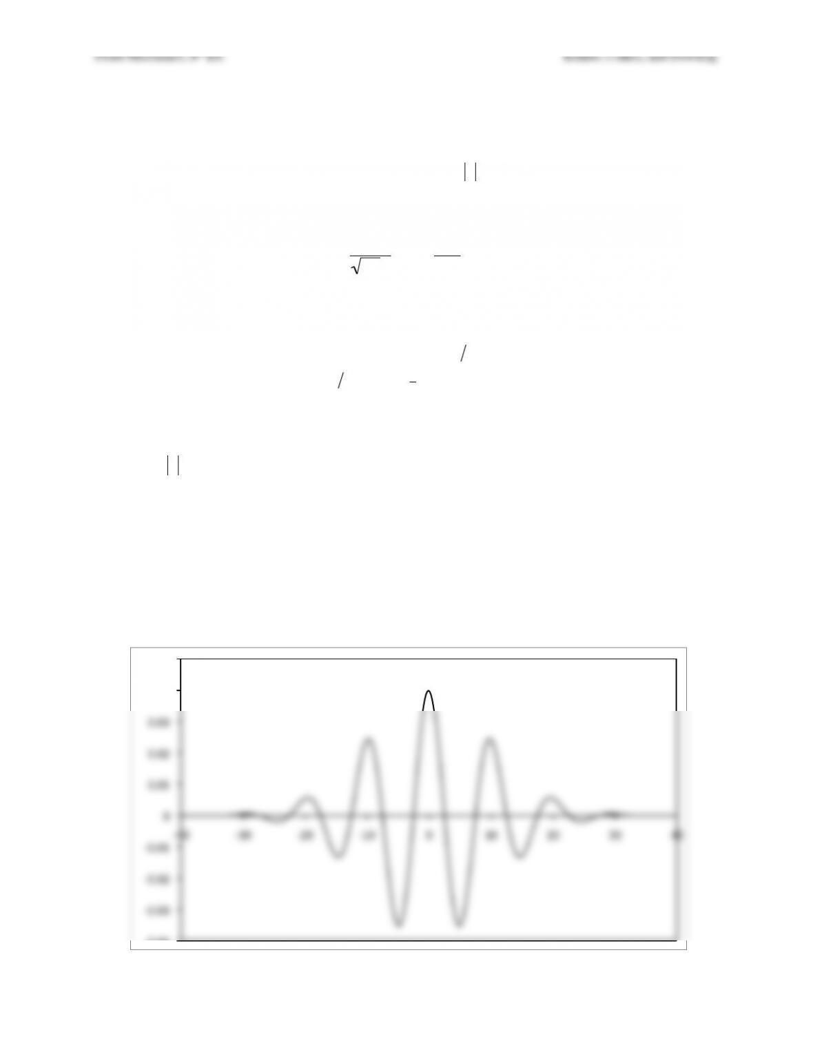
Solution 8.13. a) Below is a plot of Re{
η
(x,0)} vs. x for |x| ≤ 40 m when
α
= 10 m and kd = 2π/
λ
d
= 2π/10 m–1.
!”#”$%
!”#”&%
!”#”‘%
!”#”(%
“%
“#”(%
“#”‘%
“#”&%
“#”$%
“#”)%
!$”% !&”% !'”% !(“% “% (“% ‘”% &”% $”%

Fluid Mechanics, 6th Ed. Kundu, Cohen, and Dowling
b) Start from the given formula for
˜
η
(k)
, and insert the given initial wave form
η
(x,0):
˜
η
(k)=1
2
πη
(x,0)exp −ikx
[ ]
−∞
+∞
∫dx =1
2
π
1
2
πα
exp −x2
2
α
2+ikdx
(
)
*
+
,
–
exp −ikx
[ ]
−∞
+∞
∫dx
.
Complete the square in the exponent, and use the integration variable
β
=1
2
α
x−
α
2i(kd−k)
[ ]
to find:
˜
η
(k)=1
2
π
2
πα
exp −1
2
α
2x2−2
α
2i(kd−k)x+
α
4(kd−k)2−
α
4(kd−k)2
[ ]
&
‘
(
)
*
+
−∞
+∞
∫dx
=1
2
π
2
πα
exp −1
2
α
2x−
α
2i(kd−k)
[ ]
2−
α
2(kd−k)2
2
&
‘
(
)
*
+
−∞
+∞
∫dx
=1
2
π
2
πα
exp −
α
2(kd−k)2
2
&
‘
(
)
*
+ 2
α
exp −
β
2
{ }
−∞
+∞
∫d
β
=1
2
π
exp −
α
2(kd−k)2
2
&
‘
(
)
*
+
,
where the final definite integral over b is
π
. Below is a plot of
˜
η
(k)
vs. k for when
α
= 10 m
and kd = 2π/
λ
d = 2π/10 m–1 ≈ 0.628 m–1. Clearly the wave-packet carries most of its energy in
wave numbers near kd, and
˜
η
(k)
is negligible outside 0.2 < k < 1.0.
c) From the plot above, only positive wave numbers will matter because
˜
η
(k)
is small away
from kd, so the absolute value can be dropped from k in the formula for the phase. Thus, the
stationary phase wave number ks is determined from:
d
dk Φ
( )
k=ks
=d
dk kx −gk
( )
1/ 2 t
( )
k=ks
=x−1
2
g
ks
t=0
.
Solving for ks produces:
ks=gt24x2
.
d) Thus, at time t, the dominant portion of the wave packet plotted in part a) will reside at a
location x determined from:
ks=kd=gt24x2
, and this location is:
x=1
2g kdt
. Therefore, the
propagation speed, x/t, of the dominant portion of the wave packet is the group speed,
!”
!#!$”
!#!%”
!#!&”
!#!'”
!#(“
!#($”
!#(%”
!#(&”
!” !#$” !#%” !#&” !#'” (“ (#$” (#%”
Fluid Mechanics, 6th Ed. Kundu, Cohen, and Dowling
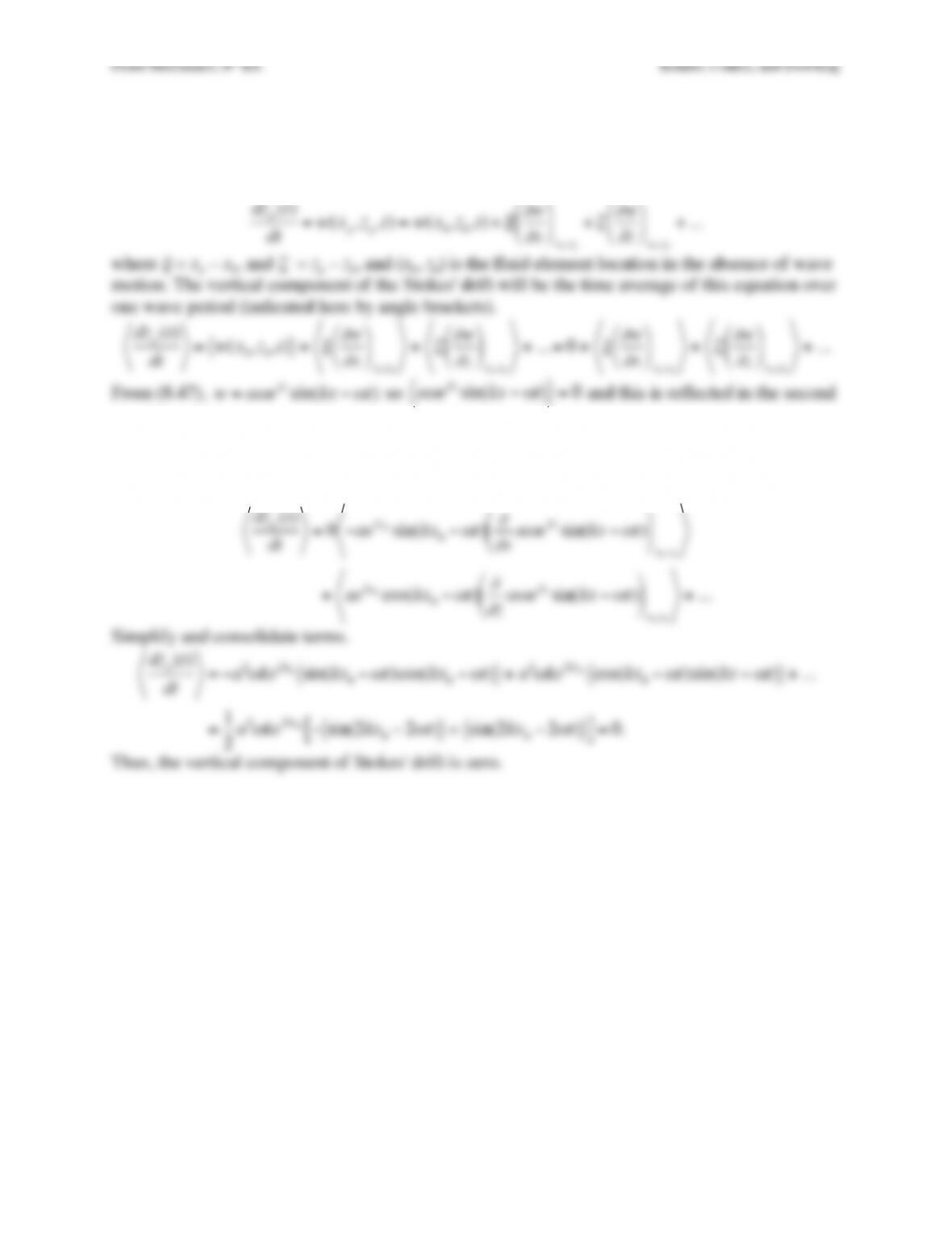
Exercise 8.14. Show that the vertical component of the Stokes’ drift is zero.
Solution 8.14. Start with the vertical-direction particle velocity equation (8.84b) expanded to
include first order-variations in both fluid velocity components.
dzp(t)
dt =w(xp,zp,t)=w(x0,z0,t)+
ξ∂
w
∂
x
$
%
& ‘
(
)
x0,z0
+
ζ∂
w
∂
z
$
%
& ‘
(
)
x0,z0
+…
where
ξ
= xp – x0, and
ζ
= zp – z0, and (x0, z0) is the fluid element location in the absence of wave
motion. The vertical component of the Stokes’ drift will be the time average of this equation over
one wave period (indicated here by angle brackets).
dzp(t)
dt =w(x0,z0,t)+
ξ∂
w
∂
x
$
%
& ‘
(
)
x0,z0
+
ζ∂
w
∂
z
$
%
& ‘
(
)
x0,z0
+… =0+
ξ∂
w
∂
x
$
%
& ‘
(
)
x0,z0
+
ζ∂
w
∂
z
$
%
& ‘
(
)
x0,z0
+…
From (8.47),
w=a
ω
ekz sin(kx −
ω
t)
so
a
ω
ekz sin(kx −
ω
t)=0
and this is reflected in the second
equality above. The two time averages involving displacements and velocity gradients can be
calculated using the deep-water ka << 1 results for
ξ
,
ζ
, u, and w given by (8.46) and (8.47):
ξ
≅ −aekz0sin(kx0−
ω
t)
,
ζ
≅aekz0cos(kx0−
ω
t)
, and
u=a
ω
ekz cos(kx −
ω
t)
,
plus the result for w given above. Substituting in these relationships produces:
dzp(t)
dt =0−aekz0sin(kx0−
ω
t)
∂
∂
xa
ω
ekz sin(kx −
ω
t)
%
&
‘ (
)
*
x0,z0
+aekz0cos(kx0−
ω
t)
∂
∂
za
ω
ekz sin(kx −
ω
t)
%
&
‘ (
)
*
x0,z0
+…
Simplify and consolidate terms.
dzp(t)
dt =−a2
ω
ke2k0sin(kx0−
ω
t)cos(kx0−
ω
t)+a2
ω
ke2kz0cos(kx0−
ω
t)sin(kx −
ω
t)+…
=1
2a2
ω
ke2kz0−sin(2kx0−2
ω
t)+sin(2kx0−2
ω
t)
[ ]
=0.
Thus, the vertical component of Stokes’ drift is zero.
Fluid Mechanics, 6th Ed. Kundu, Cohen, and Dowling
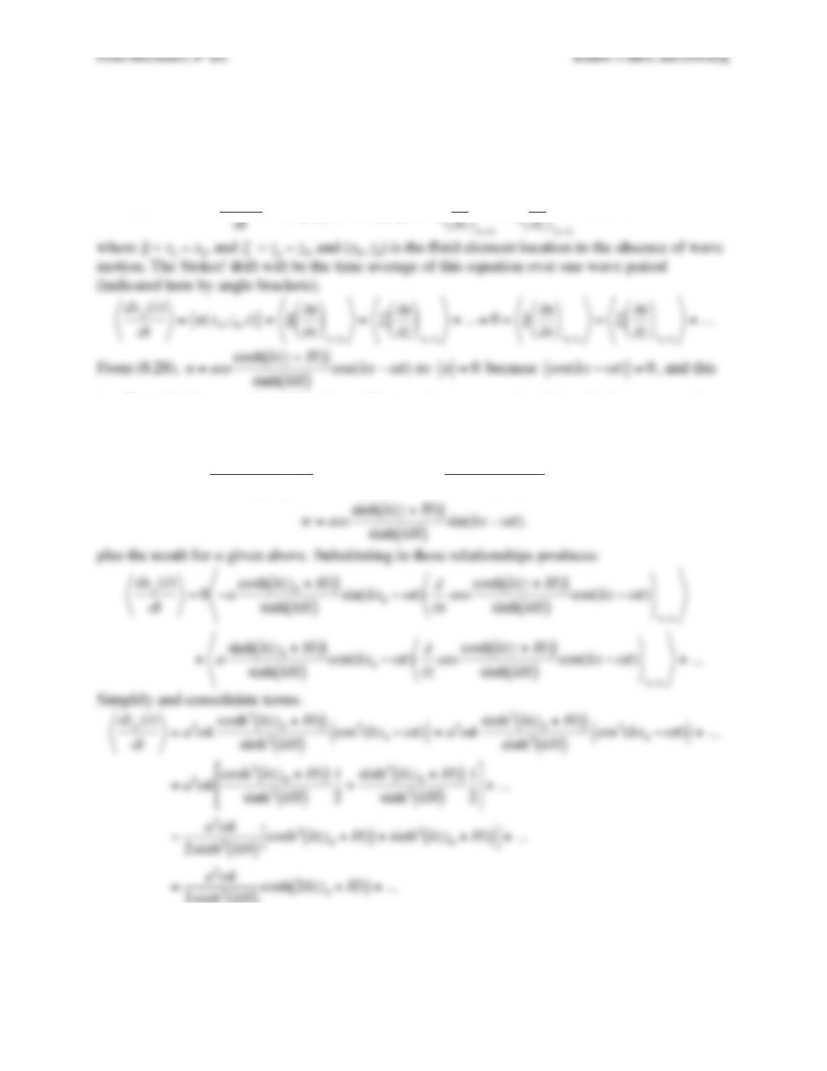
Exercise 8.15. Extend the deep water Stokes’ drift result (8.85) to arbitrary depth to derive
(8.86).
Solution 8.15. Start with the horizontal-direction particle velocity equation (8.84a) expanded to
include first order-variations in both fluid velocity components.
dxp(t)
dt =u(xp,zp,t)=u(x0,z0,t)+
ξ∂
u
∂
x
$
%
& ‘
(
)
x0,z0
+
ζ∂
u
∂
z
$
%
& ‘
(
)
x0,z0
+…
,
where
ξ
= xp – x0, and
ζ
= zp – z0, and (x0, z0) is the fluid element location in the absence of wave
is reflected in the second equality above. The two time averages involving displacements and
velocity gradients can be calculated using the deep-water ka << 1 results for
ξ
,
ζ
, u, and w given
by (8.27) and (8.35):
ξ
≅ −acosh k(z0+H)
( )
sinh kH
( )
sin(kx0−
ω
t)
,
ζ
≅asinh k(z0+H)
( )
sinh kH
( )
cos(kx0−
ω
t)
, and
w=a
ω
sinh k(z+H)
( )
sinh kH
( )
sin(kx −
ω
t)
.
plus the result for u given above. Substituting in these relationships produces:
dxp(t)
dt =0−acosh k(z0+H)
( )
sinh kH
( )
sin(kx0−
ω
t)
∂
∂
xa
ω
cosh k(z+H)
( )
sinh kH
( )
cos(kx −
ω
t)
%
&
‘
(
)
*
x0,z0
+asinh k(z0+H)
( )
sinh kH
( )
cos(kx0−
ω
t)
∂
∂
za
ω
cosh k(z+H)
( )
sinh kH
( )
cos(kx −
ω
t)
%
&
‘
(
)
*
x0,z0
+…
Simplify and consolidate terms.
dzp(t)
dt =a2
ω
kcosh2k(z0+H)
( )
sinh2kH
( )
cos2(kx0−
ω
t)+a2
ω
ksinh2k(z0+H)
( )
sinh2kH
( )
cos2(kx0−
ω
t)+…
=a2
ω
kcosh2k(z0+H)
( )
sinh2kH
( )
1
2+sinh2k(z0+H)
( )
sinh2kH
( )
1
2
$
%
&
‘
(
)
+…
=a2
ω
k
2sinh2kH
( )
cosh2k(z0+H)
( )
+sinh2k(z0+H)
( )
[ ]
+…
=a2
ω
k
2sinh2kH
( )
cosh 2k(z0+H)
( )
+…
The final result is (8.86).
Fluid Mechanics, 6th Ed. Kundu, Cohen, and Dowling
Exercise 8.16. Explicitly show through substitution and differentiation that (8.88) is a solution of
(8.87).
Solution 8.16. Equation (8.87) involves time and space differentiations of (8.88). Let
γ
=3a4H3
( )
1 2
to save a little writing. The necessary derivatives are:
∂η
∂
t=
∂
∂
t
acosh23a4H3
( )
1 2 (x−ct)
{ }
%
&
‘ (
)
* =−2asinh
γ
(x−ct)
{ }
(−
γ
c)
cosh3
γ
(x−ct)
{ }
=2a
γ
csinh
γ
(x−ct)
{ }
cosh3
γ
(x−ct)
{ }
,
∂η
∂
x=
∂
∂
x
a
cosh2
γ
(x−ct)
&
( )
+ =−2asinh
γ
(x−ct)
{ }
(
γ
)
cosh3
γ
(x−ct)
=−2a
γ
sinh
γ
(x−ct)
{ }
cosh3
γ
(x−ct)
,
=−2a
γ
2cosh2
cosh4
γ
(x−ct)
{ }
‘
( )
*
+ =−2a
γ
21−2sinh2
cosh4
γ
(x−ct)
{ }
‘
( )
*
+
,
and
∂
3
η
∂
x3=−2a
γ
2
∂
∂
x
1−2sinh2
γ
(x−ct)
{ }
cosh4
γ
(x−ct)
{ }
&
‘
( )
*
+
=−2a
γ
3−4 sinh
γ
(x−ct)
{ }
cosh
γ
(x−ct)
{ }
cosh4
γ
(x−ct)
{ }
−41−2sinh2
γ
(x−ct)
{ }
( )
sinh
γ
(x−ct)
{ }
cosh5
γ
(x−ct)
{ }
&
‘
(
(
)
*
+
+
=8a
γ
3sinh
γ
(x−ct)
{ }
cosh2
γ
(x−ct)
{ }
cosh5
γ
(x−ct)
{ }
+1−2sinh2
γ
(x−ct)
{ }
( )
sinh
γ
(x−ct)
{ }
cosh5
γ
(x−ct)
{ }
&
‘
(
(
)
*
+
+
=8a
γ
3sinh
γ
(x−ct)
{ }
3−cosh2
γ
(x−ct)
{ }
( )
cosh5
γ
(x−ct)
{ }
&
‘
(
(
)
*
+
+
It is now clear that the arguments of all the hyperbolic functions are the same, so, to save writing,
continue with the implicit notation that {} = {
γ
(x – ct)}. The next step is to start reconstructing
(8.87), the Korteweg-DeVries equation. Consider the first two terms together:
∂η
∂
t+c0
∂η
∂
x=2a
γ
(c−c0)sinh
{ }
cosh3
{ }
=a2
γ
c0
H
sinh
{ }
cosh3
{ }
,
where the final equality follows from the propagation speed relationship
c=c01+a2H
( )
. The
third and fourth terms are:
3
2
c0
η
H
∂η
∂
x+c0H2
6
∂
3
η
∂
x3=−3c0
γ
a2
H
sinh
{ }
cosh5
{ }
+4c0H2
3
a
γ
3sinh
{ }
3−cosh2
{ }
( )
cosh5
{ }
&
‘
(
(
)
*
+
+
=−3c0
γ
a2
H+4c0H2
3
3a
4H3
,
–
. /
0
1
3a
γ
&
‘
( )
*
+ sinh
{ }
cosh5
{ }
−4c0H2
3
3a
4H3
,
–
. /
0
1
a
γ
sinh
{ }
cosh3
{ }
&
‘
( )
*
+
,
Fluid Mechanics, 6th Ed. Kundu, Cohen, and Dowling
Fluid Mechanics, 6th Ed. Kundu, Cohen, and Dowling
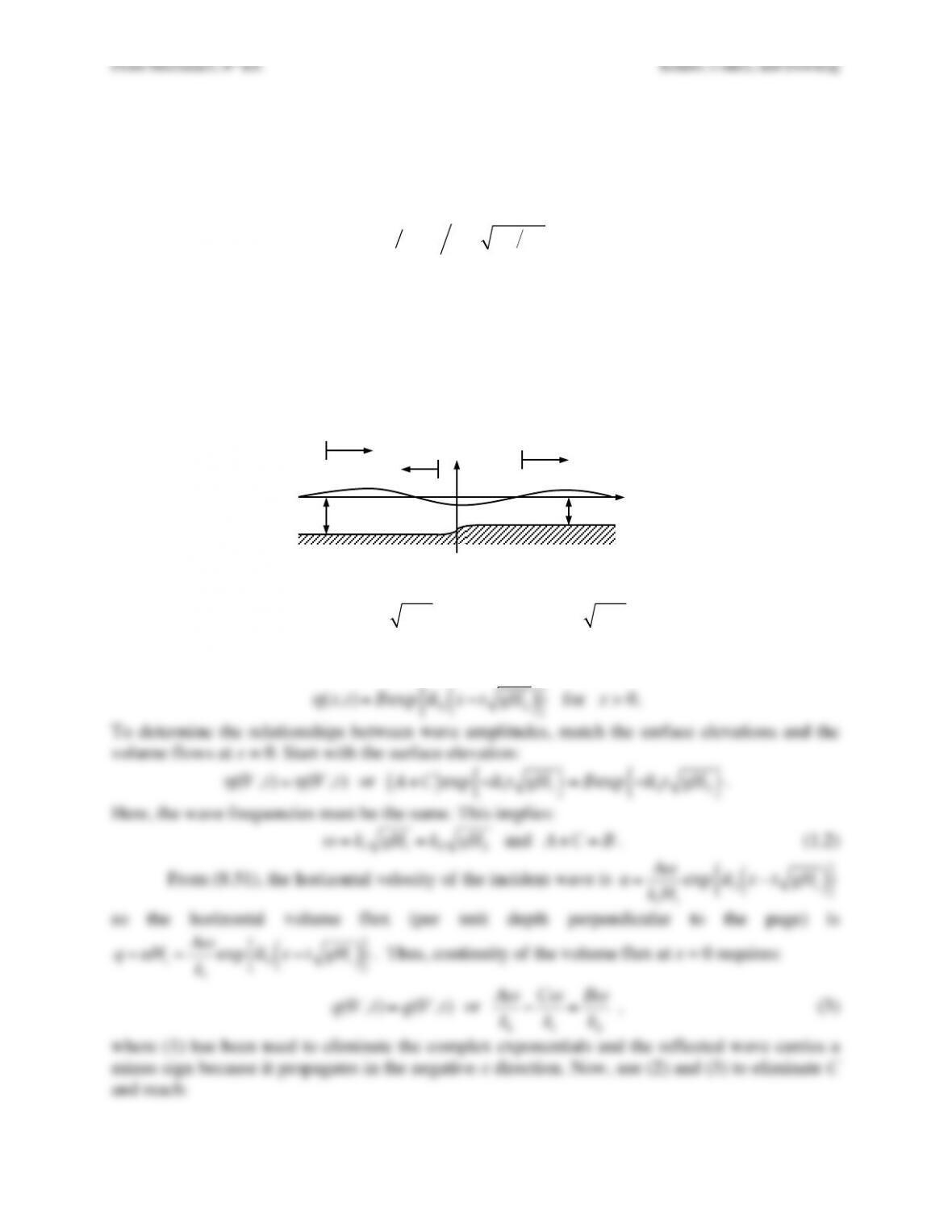
Exercise 8.17. A sinusoidal long-wavelength shallow-water wave with amplitude A and wave
number k1 = 2
π
/
λ
1 travels to the right in water of depth H1 until it encounters a mild depth
transition at x = 0 to a slightly shallower depth H2. A portion of the incident wave continues to
the right with amplitude B and a portion is reflected and propagates to the left.
a) By requiring the water surface deflection and the horizontal volume flux in the water column
to be continuous at x = 0, show that
B A =2 1+H2H1
( )
.
b) If a tsunami wave starts with A = 2.0 m in water 5 km deep, estimate its amplitude when it
reaches water 10 m deep if the ocean depth change can be modeled as a large number of discrete
depth changes. [Recommendation: consider multiple steps of H2/H1 = 0.90, since (0.90)59 ≈
0.002 = (10 m)/(5 km)].
c) Redo part b) when the wave’s energy flux remains constant at both depths when
λ
1 = 100 km
(as was done in Example 8.6).
d) Compare the results of parts b) and c). Which amplitude in shallow water is lower and why is
it lower?
Solution 8.17. The surface elevation on the left will involve two waves:
η
(x,t)=Aexp ik1x−t gH1
( )
{ }
+Cexp ik1−x−t gH1
( )
{ }
for x < 0,
where C is the amplitude of the reflected wave. The surface elevation on the right will only
involve the transmitted wave with amplitude B:
η
(x,t)=Bexp ik2x−t gH2
( )
{ }
for x > 0.
To determine the relationships between wave amplitudes, match the surface elevations and the
volume flows at x = 0. Start with the surface elevation:
η
(0−,t)=
η
(0+,t)
or
A+C
( )
exp −ik1t gH1
{ }
=Bexp −ik2t gH2
{ }
.
Here, the wave frequencies must be the same. This implies:
ω
=k1gH1=k2gH2
and
A+C=B
. (1,2)
From (8.51), the horizontal velocity of the incident wave is
u=A
ω
k1H1
exp ik1x−t gH1
( )
{ }
so the horizontal volume flux (per unit depth perpendicular to the page) is
q=uH1=A
ω
k1
exp ik1x−t gH1
( )
{ }
. Thus, continuity of the volume flux at x = 0 requires:
q(0−,t)=q(0+,t)
or
A
ω
k1
−C
ω
k1
=B
ω
k2
, (3)
where (1) has been used to eliminate the complex exponentials and the reflected wave carries a
minus sign because it propagates in the negative-x direction. Now, use (2) and (3) to eliminate C
and reach:
x!
z!
H1!
H2!
A!B!
Fluid Mechanics, 6th Ed. Kundu, Cohen, and Dowling
5 km:
c=gH =(9.81ms−2)(5, 000m)
= 221.5 ms–1, ka = 2
π
a/
λ
= 2
π
(2.0m)/(100km) =
1.257 ×10⁻⁴
.
Here a/H =
4.0 ×10⁻⁴
and ka are both small enough to use linear wave results. So, from (8.44),
the energy flux, EF, for these shallow water waves is:
Fluid Mechanics, 6th Ed. Kundu, Cohen, and Dowling
Exercise 8.18. A thermocline is a thin layer in the upper ocean across which water temperature
and, consequently, water density change rapidly. Suppose the thermocline in a very deep ocean
is at a depth of 100 m from the ocean surface, and that the temperature drops across it from 30 to
20 °C. Show that the reduced gravity is g% = 0.025 m/s2. Neglecting Coriolis effects, show that
the speed of propagation of long gravity waves on such a thermocline is 1.58 m/s.
Solution 8.18. This is the case of an internal wave at the interface between a shallow layer
overlying an infinitely deep fluid (Section 8.7). Here the layer depth is 100 m, the temperature
Fluid Mechanics, 6th Ed. Kundu, Cohen, and Dowling
Exercise 8.19. Consider internal waves in a continuously stratified fluid of buoyancy frequency
N = 0.02 s–1 and average density 800 kg/m3. What is the direction of ray paths if the frequency of
oscillation is
ω
= 0.01 s–1? Find the energy flux per unit area if the amplitude of the vertical
velocity is
ˆ
w
= 1 cm/s and the horizontal wavelength is
π
meters.
Solution 8.19. Here, N = 0.02 s–1,
ω
= 0.01 s–1, k = 2π/
λ
= 2 m–1,
ˆ
w
= 1 cm/s, and
ρ
o = 800
kg/m3. From (8.138),
ω
= Ncos
θ
, solve for the angle:
θ
=cos−1
ω
N
( )
=cos−10.01 0.02
( )
=60°
.
To determine the energy flux, calculate the vertical wave number:
m = ktan
θ
= 2tan(60°) = 3.464 m–1,
and use (8.158)
F=
ρ
0
ω
mˆ
w
2
2k2ex
m
k−ez
%
&
‘ (
)
* =800(0.01)(3.464)(0.01)2
2(2)2ex
3.464
2−ez
%
&
‘ (
)
*
=3.464 ×10−41.732ex−ez
( )
W/m2.
The magnitude of the energy flux is:
F=3.464 ×10−41.7322+1
( )
1 2 =6.92 ×10⁻⁴W/m2.
Fluid Mechanics, 6th Ed. Kundu, Cohen, and Dowling
Exercise 8.20. Consider internal waves at a density interface between two infinitely deep fluids,
and show that the average kinetic energy per unit horizontal area is Ek = (
ρ
2 −
ρ
1)ga2/4.
Solution 8.20. From Section 8.7, the velocity potentials above and below the interface are:
φ
1=i
ω
a
k
e−kz exp i(kx −
ω
t)
{ }
, and
φ
2=−i
ω
a
k
e+kz exp i(kx −
ω
t)
{ }
.
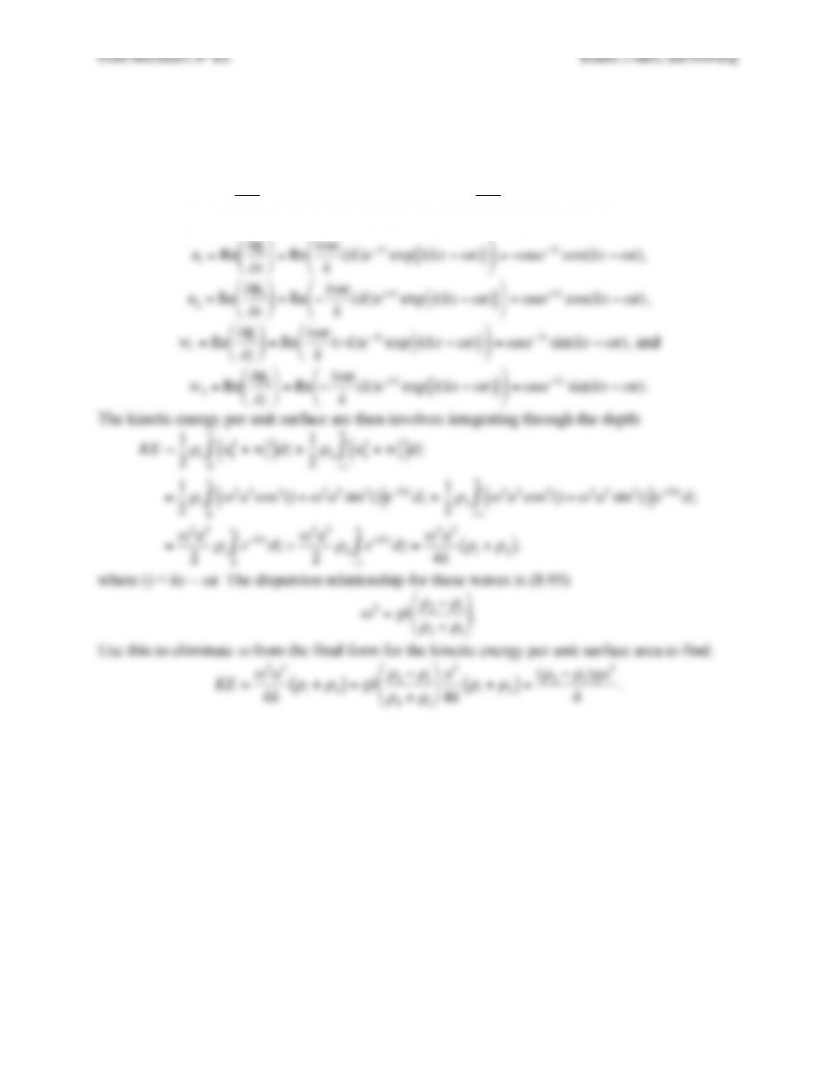
respectively. The (real) velocity components are:
u1=Re
∂φ
1
∂
x
$
%
& ‘
(
) =Re i
ω
a
k(ik)e−kz exp i(kx −
ω
t)
{ }
$
%
& ‘
(
) =−
ω
ae−kz cos(kx −
ω
t)
,
u2=Re
∂φ
2
∂
x
$
%
& ‘
(
) =Re −i
ω
a
k(ik)e+kz exp i(kx −
ω
t)
{ }
$
%
& ‘
(
) =
ω
ae+kz cos(kx −
ω
t)
,
w1=Re
∂φ
1
∂
z
$
%
& ‘
(
) =Re i
ω
a
k(−k)e−kz exp i(kx −
ω
t)
{ }
$
%
& ‘
(
) =
ω
ae−kz sin(kx −
ω
t)
, and
w2=Re
∂φ
2
∂
z
$
%
& ‘
(
) =Re −i
ω
a
k(k)e+kz exp i(kx −
ω
t)
{ }
$
%
& ‘
(
) =
ω
ae+kz sin(kx −
ω
t)
.
The kinetic energy per unit surface are then involves integrating through the depth:
KE =1
2
ρ
1u1
2+w1
2
( )
0
∞
∫dz +1
2
ρ
2u2
2+w2
2
( )
−∞
0
∫dz
=1
2
ρ
1
ω
2a2cos2() +
ω
2a2sin2()
( )
0
∞
∫e−2kz dz +1
2
ρ
2
ω
2a2cos2() +
ω
2a2sin2()
( )
e+2kz
−∞
0
∫dz
=
ω
2a2
2
ρ
1e−2kz
0
∞
∫dz +
ω
2a2
2
ρ
2e+2kz
−∞
0
∫dz =
ω
2a2
4k
ρ
1+
ρ
2
( )
.
where () = kx –
ω
t. The dispersion relationship for these waves is (8.95)
ω
2=gk
ρ
2−
ρ
1
ρ
2+
ρ
1
%
&
‘
(
)
*
.
Use this to eliminate
ω
from the final form for the kinetic energy per unit surface area to find:
KE =
ω
2a2
4k
ρ
1+
ρ
2
( )
=gk
ρ
2−
ρ
1
ρ
2+
ρ
1
%
&
‘
(
)
* a2
4k
ρ
1+
ρ
2
( )
=(
ρ
2−
ρ
1)ga2
4
.
Fluid Mechanics, 6th Ed. Kundu, Cohen, and Dowling
Exercise 8.21. Consider waves in a finite layer overlying an infinitely deep fluid. Using the
constants given in (8.105) through (8.108), prove the dispersion relation (8.109).
Solution 8.21. Equations (8.105)-(8.108) are:
A=−ia
2
ω
k+g
ω
$
%
& ‘
(
)
,
B=ia
2
ω
k−g
ω
$
%
& ‘
(
)
,
C=−ia
2
ω
k+g
ω
$
%
& ‘
(
) −ia
2
ω
k−g
ω
$
%
& ‘
(
)
e2kH
, and
b=ik
ω
Ce−kH
,
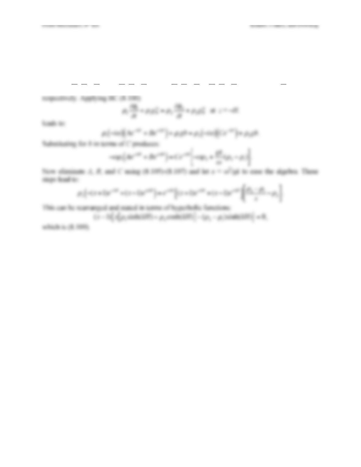
respectively. Applying BC (8.100)
Fluid Mechanics, 6th Ed. Kundu, Cohen, and Dowling
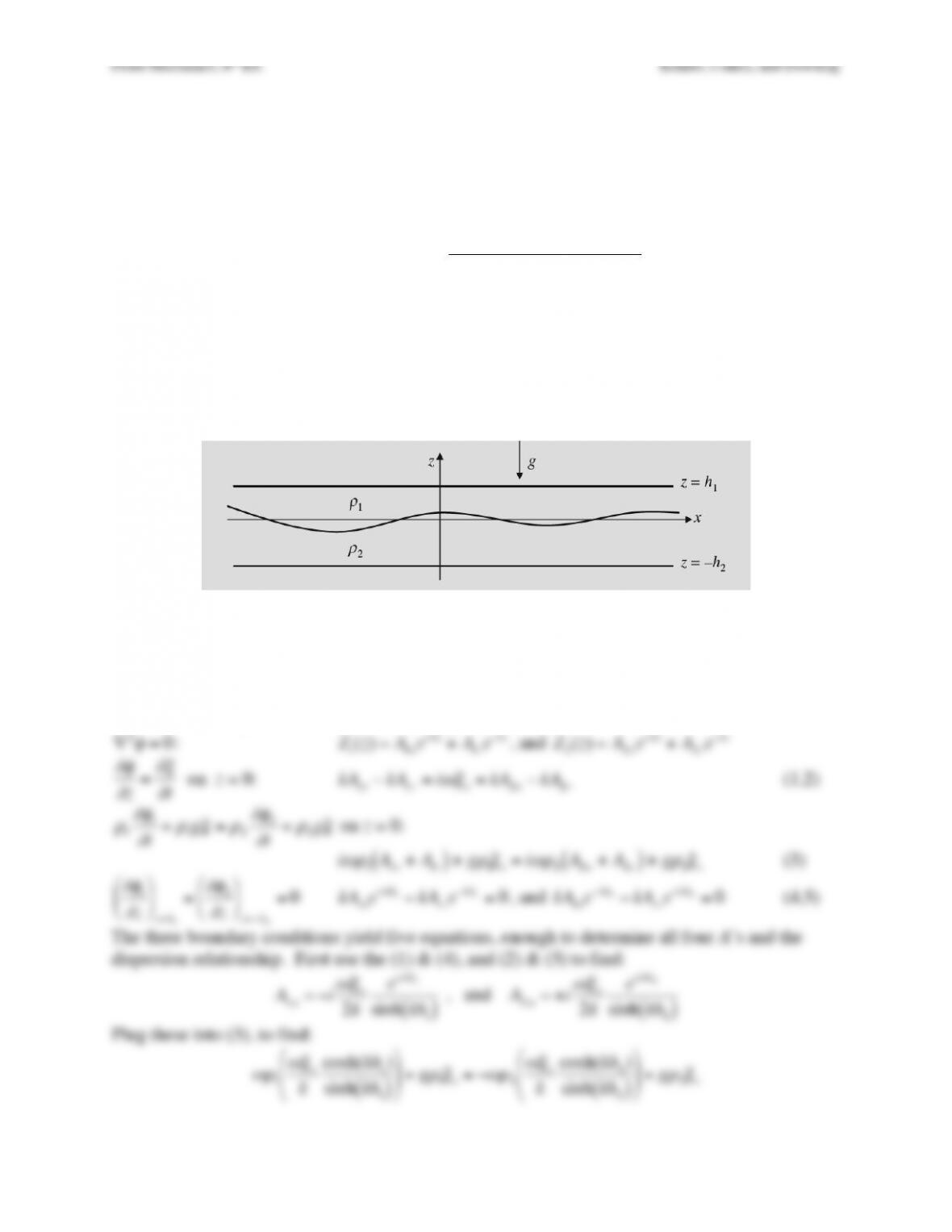
Exercise 8.22. A simple model of oceanic internal waves involves two ideal incompressible
fluids (
ρ
2 >
ρ
1) trapped between two horizontal surfaces at z = h1 and z = –h2, and having an
average interface location of z = 0. For traveling waves on the interface, assume that the
interface deflection from z = 0 is
ξ
=
ξ
oRe exp i(
ω
t−kx)
( )
{ }
. The phase speed of the waves is c =
ω
/k.
a) Show that dispersion relationship is:
ω
2=gk(
ρ
2−
ρ
1)
ρ
2coth(kh2)+
ρ
1coth(kh1)
where g is the
acceleration of gravity.
b) Determine the limiting form of c for short (i.e. unconfined) waves, kh1 and kh2 → ∞.
c) Determine the limiting form of c for long (i.e. confined) waves, kh1 and kh2 → 0.
d) At fixed wavelength
λ
(or fixed k = 2π/
λ
), do confined waves go faster or slower than
unconfined waves?
e) At a fixed frequency, what happens to the wavelength and phase speed as
ρ
2 –
ρ
1 → 0?
f) What happens if
ρ
2 <
ρ
1?
Solution 8.22. a) For this problem there at two velocity potentials that must be matched at the
moving interface. Based on the form of the interface wave,
ξ
=
ξ
oRe exp i(
ω
t−kx)
( )
{ }
and the
development given in the chapter, the form of the two potentials can be set:
φ
1(x,z,t)=Z1(z)ei(
ω
t−kx )
, and
φ
2(x,z,t)=Z2(z)ei(
ω
t−kx )
Here the boundary conditions and the field equation are:
∇2
φ
=0
:
Z1(z)=A1+e+kz +A1−e−kz
, and
Z2(z)=A2+e+kz +A2−e−kz
∂φ
∂
z=
∂ξ
∂
t
on z = 0:
kA
1+−kA1– =i
ωξ
o=kA2+−kA2–
(1,2)
ρ
1
∂φ
1
∂
t+
ρ
1g
ξ
=
ρ
2
∂φ
2
∂
t+
ρ
2g
ξ
on z = 0:
i
ωρ
1A1++A1−
( )
+g
ρ
1
ξ
o=i
ωρ
2A2++A2−
( )
+g
ρ
2
ξ
o
(3)
∂φ
1
∂
z
$
%
& ‘
(
)
z=h1
=
∂φ
2
∂
z
$
%
& ‘
(
)
z=−h2
=0
kA
1+e+kh1−kA1–e−kh1=0
, and
kA
1+e−kh2−kA1– e+kh2=0
(4,5)
The three boundary conditions yield five equations, enough to determine all four A’s and the
dispersion relationship. First use the (1) & (4), and (2) & (5) to find:
A
1,±=−i
ωξ
o
2k
ekh1
sinh kh1
( )
, and
A2,±= +i
ωξ
o
2k
e±kh2
sinh kh2
( )
Plug these into (3), to find:
ωρ
1
ωξ
o
k
cosh(kh1)
sinh kh1
( )
%
&
‘
(
)
* +g
ρ
1
ξ
o=−
ωρ
2
ωξ
o
k
cosh(kh2)
sinh kh2
( )
%
&
‘
(
)
* +g
ρ
2
ξ
o
Fluid Mechanics, 6th Ed. Kundu, Cohen, and Dowling
Cancel the common factor of
ξ
o, simplify and rearrange:
ω
2=gk(
ρ
2−
ρ
1)
ρ
1coth(kh1)+
ρ
2coth(kh2)
.
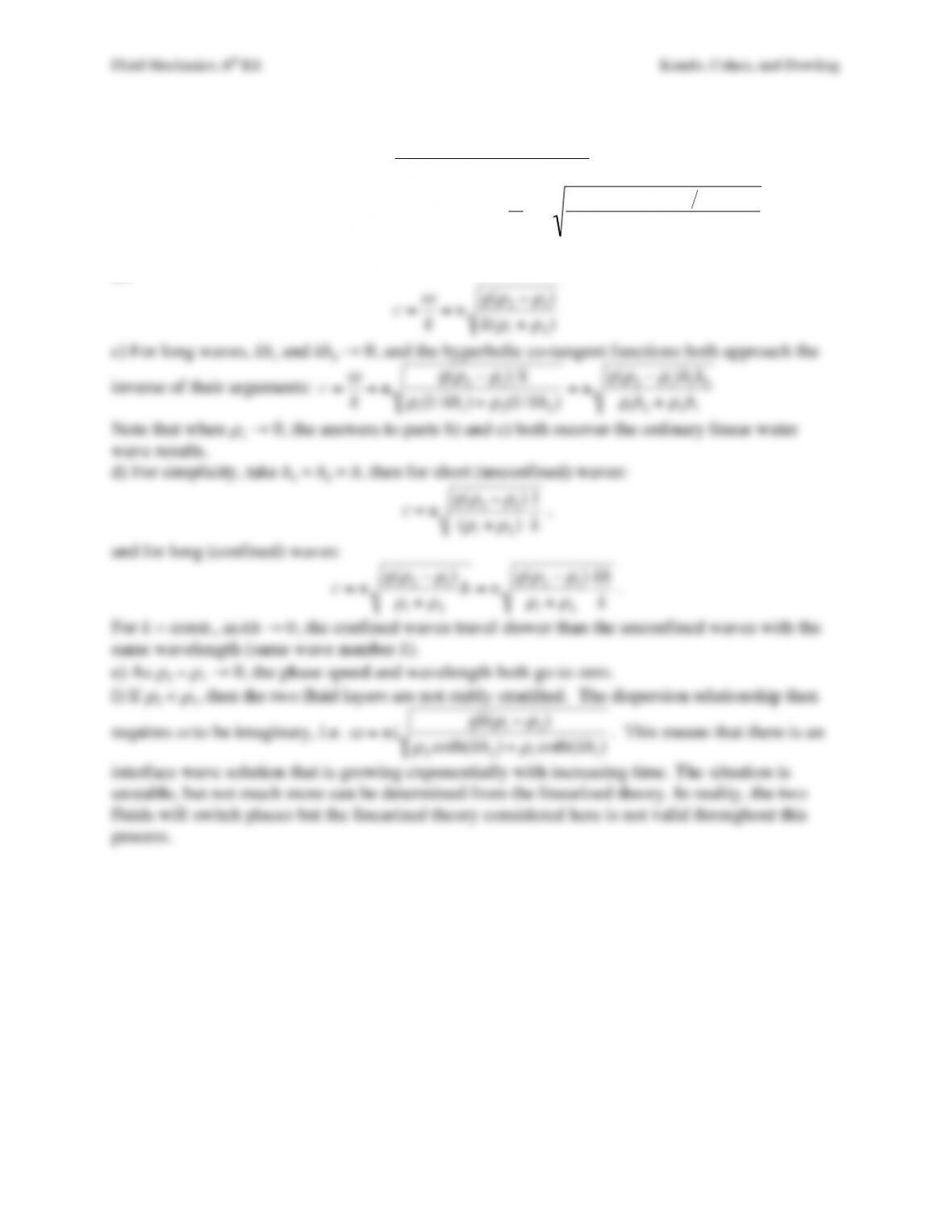
b) Using the results of part a), the phase speed is
c=
ω
k= ± g(
ρ
2−
ρ
1)k
ρ
1coth(kh1)+
ρ
2coth(kh2)
.
For short waves, kh1 and kh2 → ∞, and the hyperbolic co-tangent functions both approach unity
so:
c=
ω
k= ± g(
ρ
2−
ρ
1)
k(
ρ
1+
ρ
2)
c) For long waves, kh1 and kh2 → 0, and the hyperbolic co-tangent functions both approach the
inverse of their arguments:
c=
ω
k= ± g(
ρ
2−
ρ
1)k
ρ
1(1/ kh1)+
ρ
2(1/kh2)= ± g(
ρ
2−
ρ
1)h1h2
ρ
1h2+
ρ
2h1
Note that when
ρ
1 → 0, the answers to parts b) and c) both recover the ordinary linear water
wave results.
d) For simplicity, take h1 = h2 = h, then for short (unconfined) waves:
c= ± g(
ρ
2−
ρ
1)
(
ρ
1+
ρ
2)
1
k
,
and for long (confined) waves:
c= ± g(
ρ
2−
ρ
1)
ρ
1+
ρ
2
h= ± g(
ρ
2−
ρ
1)
ρ
1+
ρ
2
kh
k
.
For k = const., as
kh →0
, the confined waves travel slower than the unconfined waves with the
same wavelength (same wave number k).
e) As
ρ
2 –
ρ
1 → 0, the phase speed and wavelength both go to zero.
f) If
ρ
2 <
ρ
1, then the two fluid layers are not stably stratified. The dispersion relationship then
requires
ω
to be imaginary, i.e.
ω
= ±igk(
ρ
1−
ρ
2)
ρ
2coth(kh2)+
ρ
1coth(kh1)
. This means that there is an
interface wave solution that is growing exponentially with increasing time. The situation is
unstable, but not much more can be determined from the linearized theory. In reality, the two
fluids will switch places but the linearized theory considered here is not valid throughout this
process.
Fluid Mechanics, 6th Ed. Kundu, Cohen, and Dowling
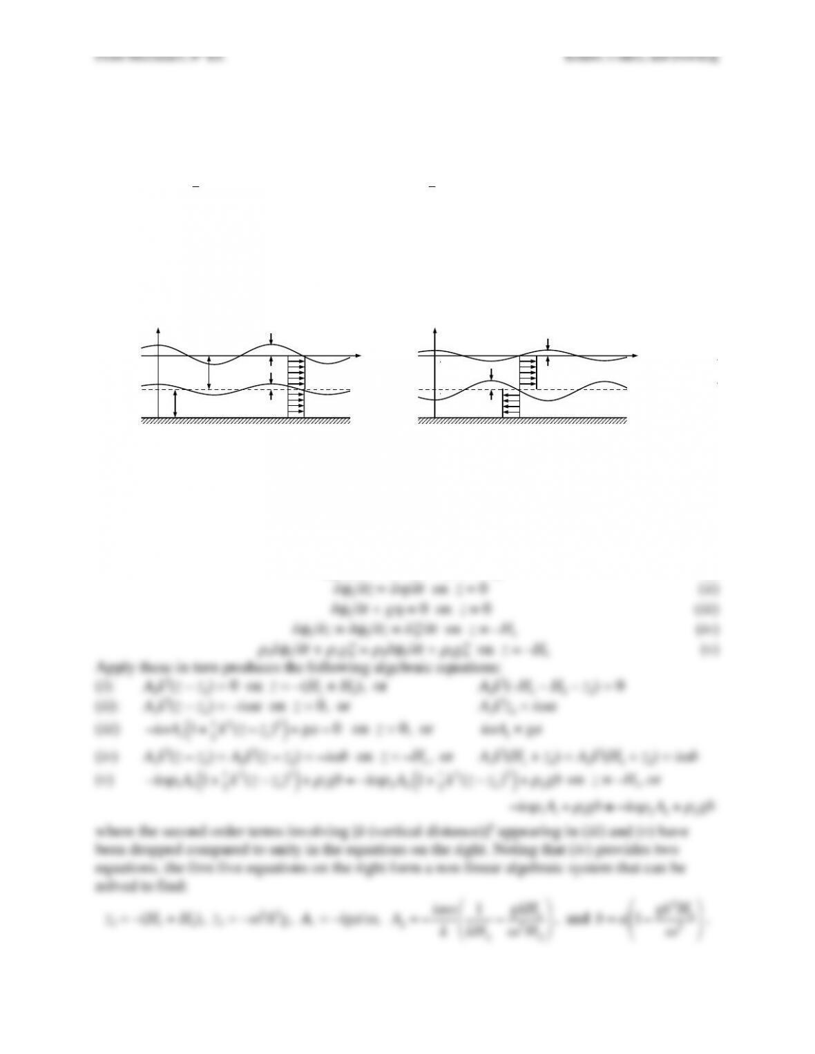
Exercise 8.23. Consider the long-wavelength limit of surface and interface waves with
amplitudes a and b, respectively, that occur when two ideal fluids with densities
ρ
1 and
ρ
2 (>
ρ
1)
are layered as shown in Figure 8.28. Here, the velocity potentials – accurate through second
order in kH1 and KH2 – in the two fluids are:
φ
1≅A11+1
2k2(z−z1)2
( )
ei(kx−
ω
t)
and
φ
2≅A21+1
2k2(z−z2)2
( )
ei(kx−
ω
t)
for kH1, KH2 << 1,
where b, A1, z1, A2, and z2 are constants to be found in terms of a, g, k,
ω
, H1 and H2. From
analysis similar to that in Section 8.7, find the dispersion relationship
ω
=
ω
(k). When H1 = H2 =
H/2, show that the surface and interface waves are in phase with a > b for the barotropic mode,
and out-of-phase with b > a for the baroclinic mode. For this case, what are the phase speeds of
the two modes? Which mode travels faster? What happens to the baroclinic mode’s phase speed
and amplitude as
ρ
2−
ρ
1→0
?
Figure 8.28.
Solution 8.23. The form of the two potentials are given in the problem statement, and the surface
and interface elevations from equilibrium can be taken from (8.101) and (8.102):
η
=aei(kx−
ω
t)
and
ζ
=bei(kx−
ω
t)
.
The boundary conditions are:
∂
φ
2/∂z = 0 on z = –(H1 + H2) (i)
∂
φ
1/∂z = ∂
η
/∂t on z = 0 (ii)
z!
b!
Barotropic!
x!
a!
H1!
H2!
ρ
1!
ρ
2!
z! a!
Baroclinic!
x!
b!
Fluid Mechanics, 6th Ed. Kundu, Cohen, and Dowling
Substitute these into the final approximate equation provided by (v):
−i
ωρ
1
−iga
ω
“
#
$%
&
‘+
ρ
1ga 1−gk2H1
ω
2
“
#
$%
&
‘≅ −i
ωρ
2
−ia
ω
k
“
#
$%
&
‘1
kH2
−gkH1
ω
2H2
“
#
$%
&
‘+
ρ
2ga 1−gk2H1
ω
2
“
#
$%
&
‘
.
Divide out the common factor of a, and simplify:
−
ρ
1
g2k2H1
ω
2≅−
ρ
2
ω
2
k
1
kH2
−gkH1
ω
2H2
#
$
%&
‘
(+
ρ
2g−
ρ
2
g2k2H1
ω
2
, or
0≅ −
ρ
2
ω
2
k2H2
+
ρ
2g1+H1
H2
#
$
%&
‘
(−
ρ
2−
ρ
1
( )
g2k2H1
ω
2
Multiply –
ω
2k2H2/
ρ
2 and rearrange to find:
0≅
ω
4−gk kH2+kH1
( )
ω
2+(
ρ
2−
ρ
1)
ρ
2
k2g2kH1kH2
.
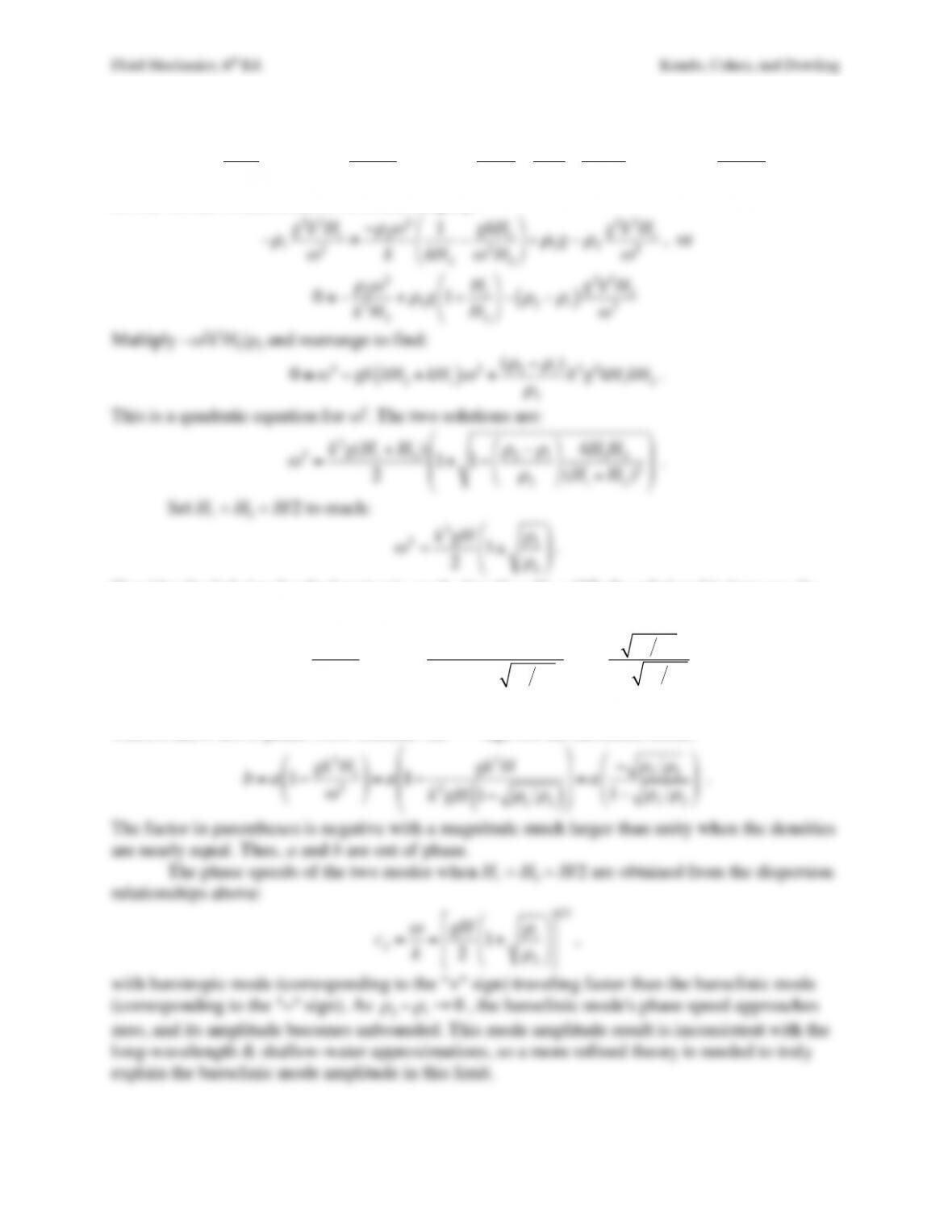
This is a quadratic equation for
ω
2. The two solutions are:
ω
2=k2g(H1+H2)
21±1−
ρ
2−
ρ
1
ρ
2
“
#
$%
&
‘4H1H2
(H1+H2)2
“
#
$
$
%
&
‘
‘
.
Set H1 = H2 = H/2 to reach:
ω
2=k2gH
2
1±
ρ
1
ρ
2
!
“
#
#
$
%
&
&
.
Consider the “+” sign for the barotropic mode. For H1 = H2 = H/2, the relationship between the
surface deflection amplitude a and the interface deflection amplitude b is:
b=a1−gk2H1
ω
2
“
#
$%
&
‘=a1−gk2H
k2gH 1+
ρ
1
ρ
2
( )
“
#
$
$
%
&
‘
‘=a
ρ
1
ρ
2
1+
ρ
1
ρ
2
“
#
$
$
%
&
‘
‘
.
The factor in parentheses is positive with a value near 1/2 when the densities are nearly equal.
Thus, a and b are in phase. Now consider the “–” sign for the baroclinic mode.
b=a1−gk2H1
ω
2
“
#
$%
&
‘=a1−gk2H
k2gH 1−
ρ
1
ρ
2
( )
“
#
$
$
%
&
‘
‘=a−
ρ
1
ρ
2
1−
ρ
1
ρ
2
“
#
$
$
%
&
‘
‘
.
The factor in parentheses is negative with a magnitude much larger than unity when the densities
are nearly equal. Thus, a and b are out of phase.
The phase speeds of the two modes when H1 = H2 = H/2 are obtained from the dispersion
relationships above:
cp=
ω
k=gH
2
1±
ρ
1
ρ
2
!
“
#
#
$
%
&
&
‘
(
)
)
*
+
,
,
1 2
,
with barotropic mode (corresponding to the “+” sign) traveling faster than the baroclinic mode
(corresponding to the “–” sign). As
ρ
2−
ρ
1→0
, the baroclinic mode’s phase speed approaches
zero, and its amplitude becomes unbounded. This mode amplitude result is inconsistent with the
long-wavelength & shallow-water approximations, so a more refined theory is needed to truly
explain the baroclinic mode amplitude in this limit.