18
ut(i,j)=u(i,j)+dt*(-0.25*(…
( (u(i+1,j)+u(i,j))^2-(u(i,j)+u(i-1,j))^2 )/dx+…
( (u(i,j+1)+u(i,j))*(v(i+1,j)+v(i,j))-…
(u(i,j)+u(i,j-1))*(v(i+1,j-1)+v(i,j-1)) )/dy )+…
Visc*((u(i+1,j)+u(i-1,j)-2*u(i,j))/dx^2+…
vv(1:Nx+1,1:Ny+1)=0.5*(v(2:Nx+2,1:Ny+1)+v(1:Nx+1,1:Ny+1));
w(1:Nx+1,1:Ny+1)=(u(1:Nx+1,2:Ny+2)-u(1:Nx+1,1:Ny+1)-…
v(2:Nx+2,1:Ny+1)+v(1:Nx+1,1:Ny+1))/(2*dx);
hold off,quiver(flipud(rot90(uu)),flipud(rot90(vv)),’r’);
hold on;contour(flipud(rot90(w)),100),axis equal,
plot(20+10*uu(20,1:Ny+1),[1:Ny+1],’k’);
plot([20,20],[1,Ny],’k’);
19
plot(60+10*uu(60,1:Ny+1),[1:Ny+1],’k’);
plot([60,60],[1,Ny],’k’); pause(0.01)
end
Notice that here we plot the velocity and the vorticity without finding the
physical location of the grid points and instead simply used that the grid is
uniform. This does, however, require us to manipulate the field slightly, since
for 2D plots, Matlab treats the first variable as the vertical one and the second
Problem 13
Extend the velocity-pressure code used to simulate the two-dimensional driven
cavity problem (Code 4) to three-dimensions. Assume that the third dimension
is unity (as the current dimensions) and take the velocity of the top wall and
the material properties to be the same. Compute the flow on a 93and 173
grids and compare the results by plotting the velocities along lines through the
center of the domain. How do the velocities in the center compare with the
two-dimensional results?
Solution
The extension of the code to three-dimensional flow is relatively straight forward.
Everything just becomes longer. The biggest difference between 2D and 3D is
that plotting the results becomes more of a challenge. Here we solve the pressure
equation using a fixed number of iterations so it may not be fully converged at
the early stages.
% Driven Cavity by the MAC Method—3D
Nx=16;Ny=16;Nz=16;Lx=1;Ly=1;Lz=1;MaxStep=50;visc=0.1;rho=1.0;
MaxIt=100; Beta=1.5; MaxErr=0.001; % parameters for SOR
dx=Lx/Nx;dy=Ly/Ny; dz=Lz/Nz; time=0.0; dt=0.002;
c(Nx+1,2,2)=1/(1/dx^2+1/dy^2+1/dz^2);
c(2,Ny+1,2) =1/(1/dx^2+1/dy^2+1/dz^2);
c(Nx+1,Ny+1,2)=1/(1/dx^2+1/dy^2+1/dz^2);
c(2,2,Nz+1) =1/(1/dx^2+1/dy^2+1/dz^2);
21
u(1:Nx+1,1:Ny+1,1)=-u(1:Nx+1,1:Ny+1,2);
u(1:Nx+1,1:Nz+1,Nz+2)=-u(1:Nx+1,1:Nz+1,Nz+1);
v(1:Nx+1,1:Ny+1,1)=-v(1:Nx+1,1:Ny+1,2);
v(1:Nx+1,1:Nz+1,Nz+2)=-v(1:Nx+1,1:Nz+1,Nz+1);
end,end,end
for i=2:Nx+1,for j=2:Ny,for k=2:Nz+1 % temp. v-velocity
vt(i,j,k)=v(i,j,k)+dt*(-0.25*(…
( (u(i,j+1,k)+u(i,j,k))*(v(i+1,j,k)+v(i,j,k))-…
(u(i-1,j+1,k)+u(i-1,j,k))*(v(i,j,k)+v(i-1,j,k)))/dx+…
22
( (w(i,j+1,k)+w(i,j,k))*(v(i,j,k+1)+v(i,j,k))-…
(w(i,j,k)+w(i,j-1,k))*(v(i,j-1,k+1)+v(i,j-1,k)) )/dy+…
((w(i,j,k+1)+w(i,j,k))^2-(w(i,j,k)+w(i,j,k-1))^2 )/dz)+…
visc*((w(i+1,j,k)+w(i-1,j,k)-2*w(i,j,k))/dx^2+…
(w(i,j+1,k)+w(i,j-1,k)-2*w(i,j,k))/dy^2+…
(w(i,j,k+1)+w(i,j,k-1)-2*w(i,j,k))/dz^2) );
end,end,end
for it=1:MaxIt % solve for pressure
for i=2:Nx+1,for j=2:Ny+1, for k=2:Ny+1
p(i,j,k)=Beta*c(i,j,k)*…
( (p(i+1,j,k)+p(i-1,j,k))/dx^2+…
(p(i,j+1,k)+p(i,j-1,k))/dy^2+…
end
% ———- Plot the final results ———————
[X,Y,Z]=ndgrid(0.5*dx:dx:1-0.5*dx, 0.5*dy:dy:1-0.5*dy,…
0.5*dz:dz:1-0.5*dz);
quiver3(X,Y,Z,u3(2:Nx+1,2:Ny+1,2:Nz+1),…
v3(2:Nx+1,2:Ny+1,2:Nz+1),w3(2:Nx+1,2:Ny+1,2:Nz+1))
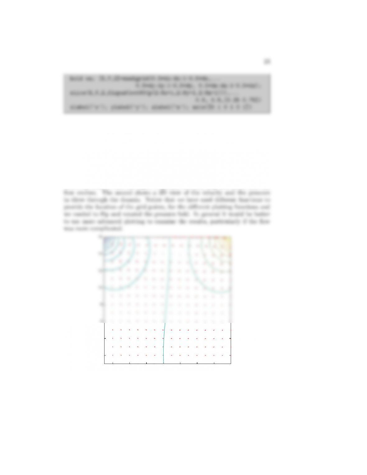
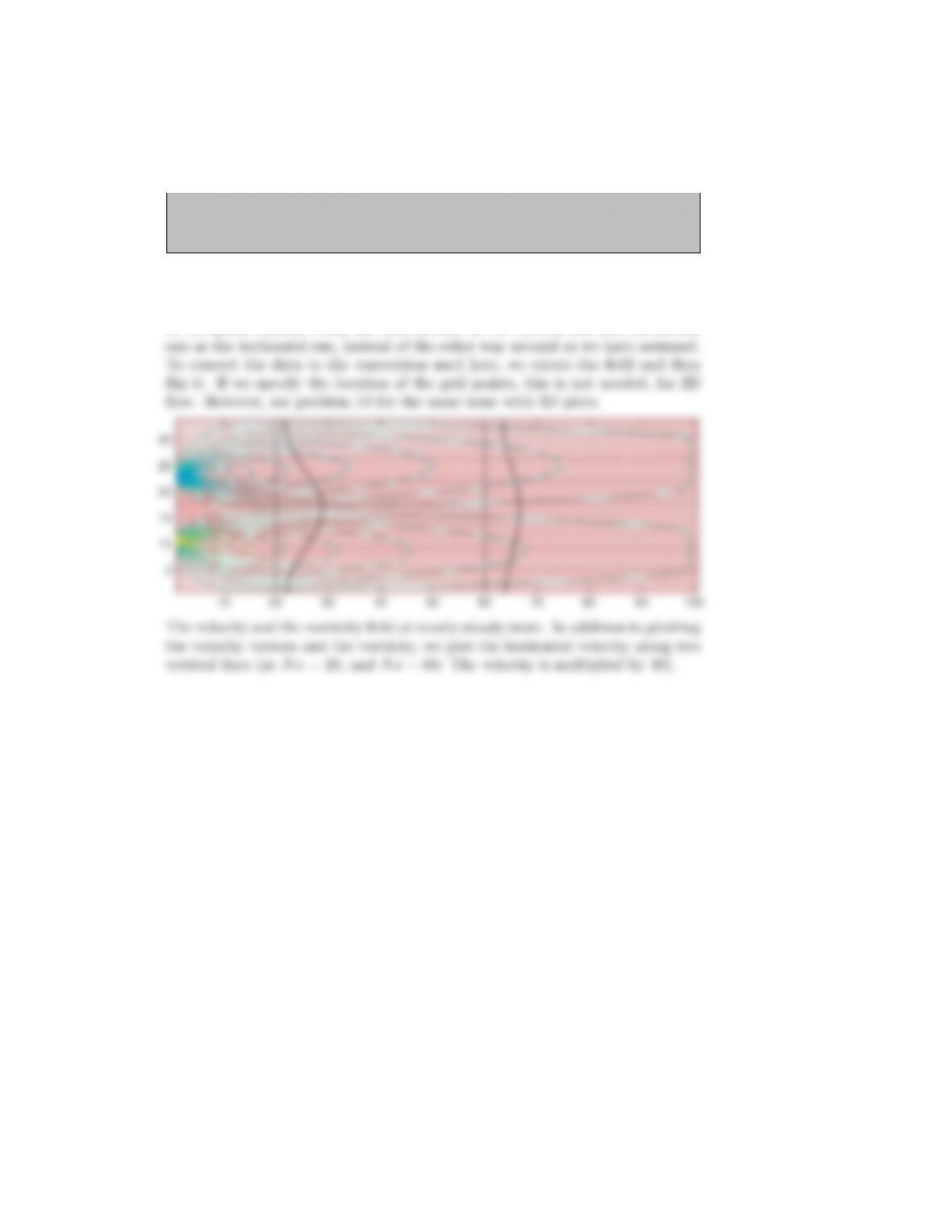
We show three figures for the results. The first one shows the velocity and the
vorticity in a plane cutting through the middle of the domain for a 173grid.
When the code is run, this figure is plotted at every step and shows how the
2 4 6 8 10 12 14 16
2
4
6
8
10
12
14
16
The velocity and the vorticity in a plane cutting through the middle of the
domain.
24
1
0.8
0.6
0.4
x
0.2
0
0
0.2
y
0.4
0.6
0.8
0.8
0
0.2
0.4
1
0.6
1
z
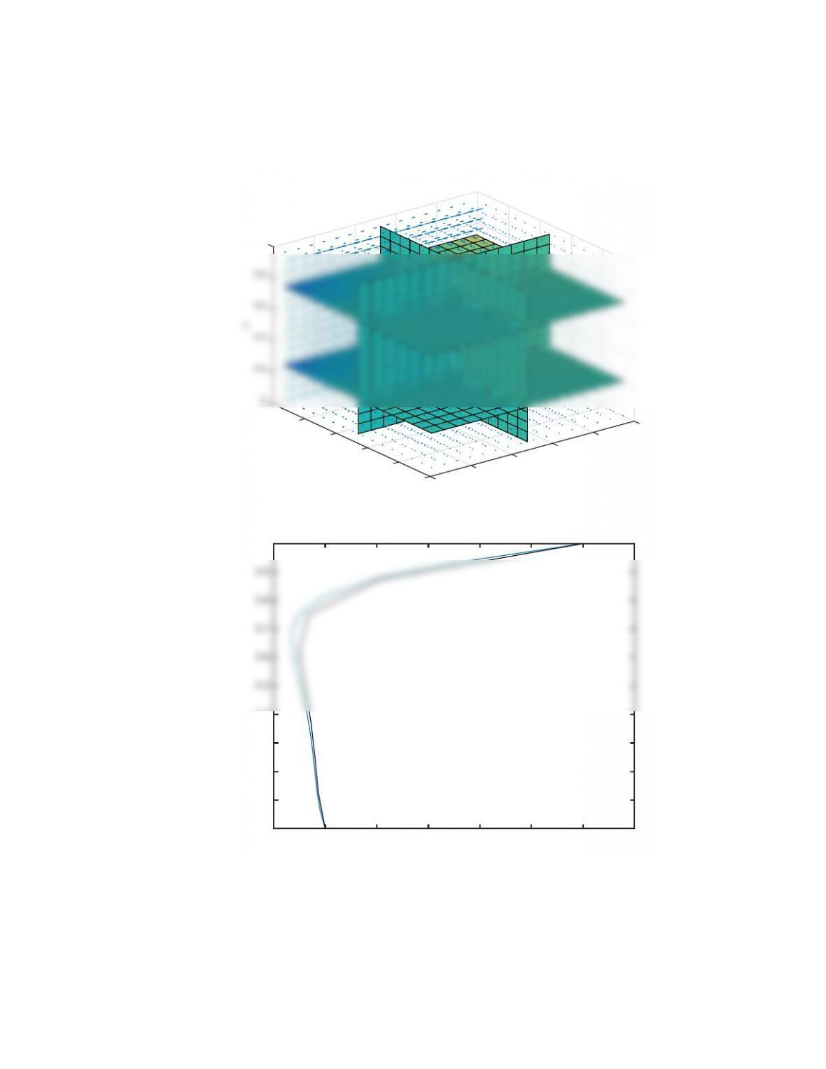
The velocity plotted using the Matlab function quiver3 and the pressure in
various planes cutting though the domain, using the Matlab function slice.
-0.2 0 0.2 0.4 0.6 0.8 1 1.2
0
0.1
0.2
0.3
0.4
0.5
0.6
0.7
0.8
0.9
1
25
Problem 14
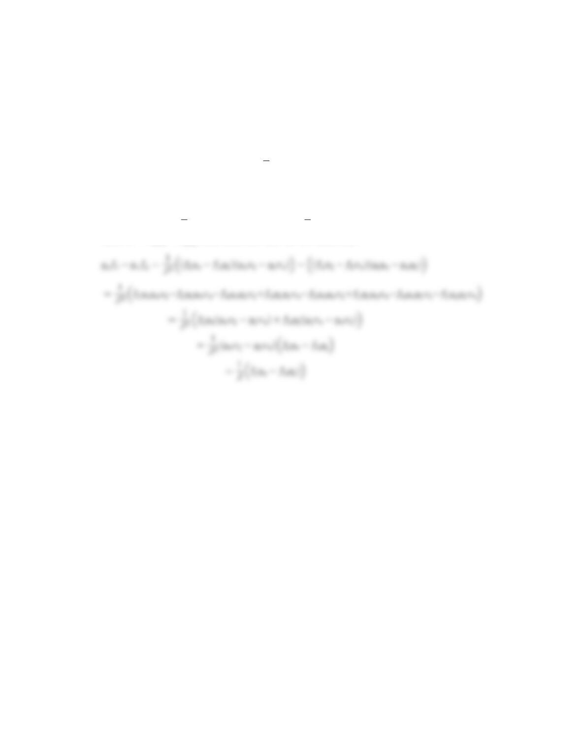
Derive equation (6.121),
gyfx−gxfy=1
J(gηfξ−gξfη).
Solution
Use that
fx=1
J(fξyη−fηyξ); and fy=1
J(fηxξ−fξxη),
where J=xξyη−xηyξ, and substitute into the left hand side:
Problem 15
Show that the equations for the first derivatives in the mapped coordinates
(equations 6.111) can be written in the so-called conservative form:
fx=1
J((fyη)ξ−(fyξ)η) and fy=1
J((fxξ)η−(fxη)ξ)
Solution
Problem 16
Derive equation (6.120),
∇2ξ=1
J3q1(xηyξξ −yηxξξ )−2q2(xηyξη −yηxξη) + q3(xηyηη −yηxηη ).
Take f=ξand use that ξη= 0 and so on.
Solution
The equation listed is actually (6.119) and we will derive that one. The deriva-
tion of (6.120) is similar. We start with
fx=1
J((fyη)ξ−(fyξ)η) where J=xξyη−xηyξ.
Expanding the terms
∇2ξ=1
J“yη
Jξyη−yη
Jηyξ−xη
Jηxξ+xη
Jξxη#=
J3“(yηξyη−yηη yξ−xηηxξ+xηξxη)J−(y2
28
Now use that J=xξyη−xηyξto get
Jξ=xξξ yη+xξyηξ −xηξyξ−xηyξξ
Jη=xξη yη+xξyηη −xηηyξ−xηyξη
Then
∇2ξ=
1
J3“xξyη(yηξyη−yηη yξ−xηηxξ+xηξxη)−xηyξ(yηξ yη−yηηyξ−xηηxξ+xηξ xη)
−(x2
η+y2
η)(xξξyη+xξyηξ −xηξyξ−xηyξξ) +
29
Problem 17
Derive numerical approximations for the velocity-pressure equations for a map-
ping where the grid lines are straight and orthogonal, but unevenly spaced.
That is, x=x(ξ) and y=y(η) only. Assume that ∆ξ= ∆η= 1. How do these
equations compare with (6.85), (6.88), (6.89), (6.90), and (6.91)?
Solution
The various relationships simplify to q1=y2
η;q2= 0; q3=x2
ξ; and J=xξyη.
The velocities are therefore
u=1
JUxξ=1
xξyηUxξ=U
yη
v=1
JV yη=1
xξyηV yη=V
xξ
.
The continuity equation is
Problem 18
When the velocity is high and diffusion is small, the linear advection-diffusion
equation can exhibit boundary layer behavior. Assume that you want to solve
(6.11) in a domain given by 0 ≤x≤1, that U > 0, and that the boundary
conditions are f(0) = 0 and f(1) = 1. The velocity Uis high and the diffusion
Dis small so we expect a boundary layer near x= 1.
(a) Sketch the solution for high Uand low D.
(b) Propose a mapping function that will cluster the grid points near the x=1
boundary.
(c) Write the equation in the mapped coordinates.
Solution
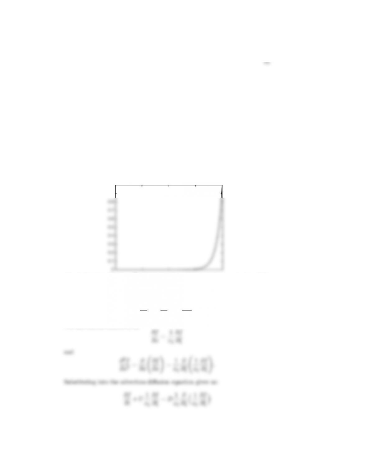
(a) This is the problem studied in section 6.2.6 and shown in figure 6.9. Here
we assume that we are solving the unsteady problem but at steady state the
solution looks like:
0
0.1
0.2
0.3
0.4
0.5
0.6
0.7
0.8
0.9
1
(b): A function like ξ=x2will cluster the points near the x= 1 part of the
domain.
(c) Start with the advection-diffusion equation
∂f
∂t +U∂f
∂x =D∂2f
∂x2.
The derivatives transform as
33
Problem 19
Derive equation (6.141).
Solution
Start with equation (6.140) and insert (6.133) and (6.134):
ˆ
Fn
j+1/2=F+(fn
j) + F−(fn
j+1) =
max(un
j,0)
ρ
ρu
ρe
n
j
+
0
p+
(pu)+
n
j
+ min(un
j+1,0)
ρ
ρu
ρe
n
j+1
+
0
p−
(pu)−
n
j+1
.
2
j+1Mn
j+1
pn
j+1cn
j+1
jMn
j
pn
jcn
j
Problem 20
Propose a numerical scheme to solve for the unsteady flow over a rectangular
cube in an unbounded domain. The Reynolds number is relatively low, 500-
1000. Identify the key issues that must be addressed and propose a solution.
Limit your discussion to one page and do NOT write down the detailed nu-
merical approximations, but state clearly what kind of spatial and temporal
discretization you would use.
Solution
The key issues and how those control the design of the numerical scheme are
listed below:
•Since the Reynolds number is relatively low, it is safe to assume that the
flow is laminar so no turbulence model is needed.