1
Chapter 6 Excercises
Problem 1
Show, by Taylor expansion, that
d3f
dx3≈fj+2 −2fj+1 + 2fj−1−fj−2
2∆x3.
What is order of this approximation?
Solution
Expand around xj:
fj+1 =fj+∂f
∂x ∆x+∂2f
∂x2
∆x2
2+∂3f
∂x3
∆x3
6+∂4f
∂x4
∆x4
24 +O(∆x5) (1)
fj−1=fj−∂f
∂x ∆x+∂2f
∂x2
∆x2
2−∂3f
∂x3
∆x3
6+∂4f
∂x4
∆x4
24 +O(∆x5) (2)
4∆x2
8∆x3
(2∆x)4
2
Problem 2
Consider the following “backward in time” approximation for the diffusion equa-
tion:
fn+1
j=fn
j+∆tD
∆x2fn+1
j+1 +fn+1
j−1−2fn+1
j
(a) Determine the accuracy of this scheme.
(b) Find its stability properties by von Neumann’s method. How does it compare
with the forward in time, centered in space approximation considered earlier?
Solution
Expand around fn+1
j
fn
j=fn+1
j−∂f
∂t ∆t+∂2f
∂t2
∆t2
2+O(∆t3)
fn+1
j+1 =fn+1
j+∂f
∂x ∆x+∂2f
∂x2
∆x2
2+∂3f
∂x3
∆x3
6+O(∆x4)
∆x2
∆x3
Problem 3
Approximate the linear advection equation
∂f
∂t +U∂f
∂x = 0 U > 0
by the backward in time method from problem 2. Use the standard second
order centered difference approximation for the spatial derivative.
(a) Write down the finite difference equation.
(b) Write down the modified equation
(c) Find the accuracy of the scheme
(d) Use the von Neuman’s method to determine the stability of the scheme.
Solution
(a) The scheme is:
fn+1
j−fn
j
∆t+Ufn+1
j−1−fn+1
j−1
2∆x= 0
(b) First expand around fn+1
j:
∆t2

Problem 4
Consider the following finite difference approximation to the diffusion equation:
fn+1
j=fn
j+ 2∆tD
∆x2fn
j+1 −fn+1
j−fn−1
j+fn
j−1.
This is the so-called Dufort-Frankel scheme, where the time integration is the
”Leapfrog” method, and the spatial derivative is the usual center difference
approximation, except that we have replaced fn
jby (1/2)(fn+1
j+fn−1
j) . Derive
the modified equation and determine the accuracy of the scheme. Are there any
surprises?
Solution
Writing
fn+1
j=fn
j+∂f
∂t ∆t+∂2f
∂t2
∆t2
2+∂3f
∂t3
∆t3
6+∂4f
∂t4
∆t4
24 +O(∆t5)
∆t2
∆t3
∆t4
Problem 5
The following finite difference approximation is given
fn+1
j=1
2(fn
j+1 +fn
j−1)−∆tU
2∆xfn
j+1 −fn
j−1
(a) Write down the modified equation
(b) What equation is being approximated?
(c) Determine the accuracy of the scheme
(d) Use the von Neuman’s method to examine under which conditions this
scheme is stable.
Solution
(a) Start by expanding
fn+1
j=fn
j+∂f
∂t ∆t+∂2f
∂t2
∆t2
2+O(∆t3)
fn
j+1 =fn
j+∂f
∂x ∆x+∂2f
∂x2
∆x2
2+∂3f
∂x3
∆x3
6+O(∆x4)
∆x2
∆x3
Problem 6
Consider the equation ∂f
∂t =g(f),
and the second-order predictor-corrector method:
f∗
j=fn
j+ ∆tg(fn)
fn+1
j=fn
j+∆t
2(g(fn) + g(f∗)).
Show that this method can also be written as:
f∗
j=fn
j+ ∆tg(fn)
f∗∗
j=f∗
j+ ∆tg(f∗)
fn+1
j= (1/2)(fn+f∗∗).
That is, you simply take two explicit Euler steps and then average the solution
at the beginning of the time step and the end. This makes it particularly simple
to extend a first order explicit time integration scheme to second order.
Solution
The first equations in each formulation are the same. To show that the second
two equations in the second formulation are the same as the final equation of
the first formulation, substitute the second and first equation into the third one:
2(∆tg(fn
Problem 7
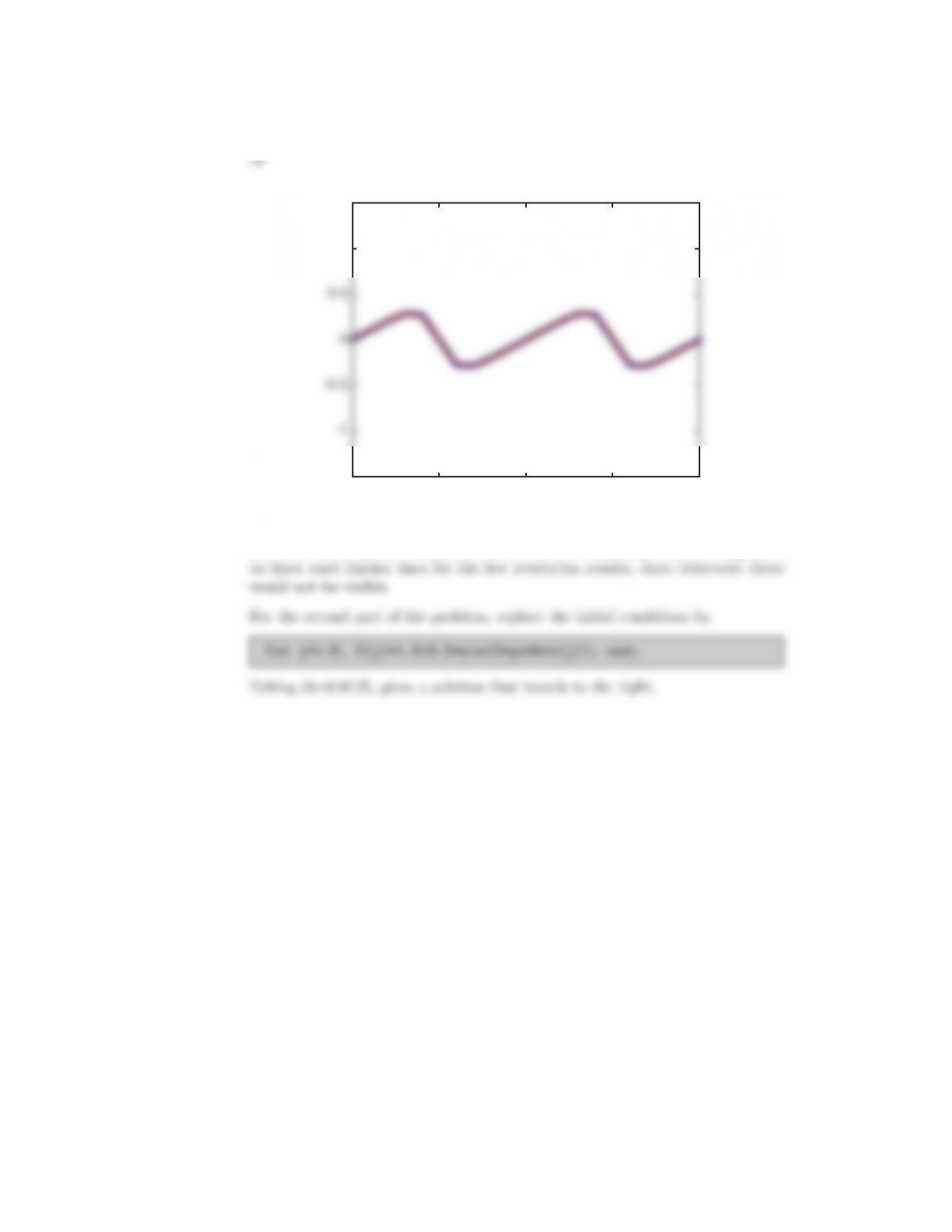
Modify the code used to solve the one-dimensional linear advection equation
(Code 1) to solve the Burgers equation:
∂f
∂t +∂
∂xf2
2=D∂2f
∂x2
using the same initial conditions. What happens? Refine the grid. How does
the solution change if we add a constant (say 1) to the initial conditions?
Solution
The modified code is:
% one-dimensional NONLINEAR advection-diffusion
% by the FTCS scheme
N=21; nstep=10; L=2.0; dt=0.05;D=0.05; k=1;
dx=L/(N-1); for j=1:N, x(j)=dx*(j-1);end
f=zeros(N,1); fo=zeros(N,1); time=0.0;
for j=1:N, f(j)=0.5*sin(2*pi*k*x(j)); end;
for m=1:nstep, m, time
0 0.5 1 1.5 2
-1.5
-1
-0.5
0
0.5
1
1.5
Running the code for for three different resolutions N= 21,41,81 with dt =
0.05,0.025,0.0125 up to time 0.25 (for 5,10,20) steps, produces the figure above.
Even for the coarsest resolution, the solution is essentially fully converged, so
Problem 8
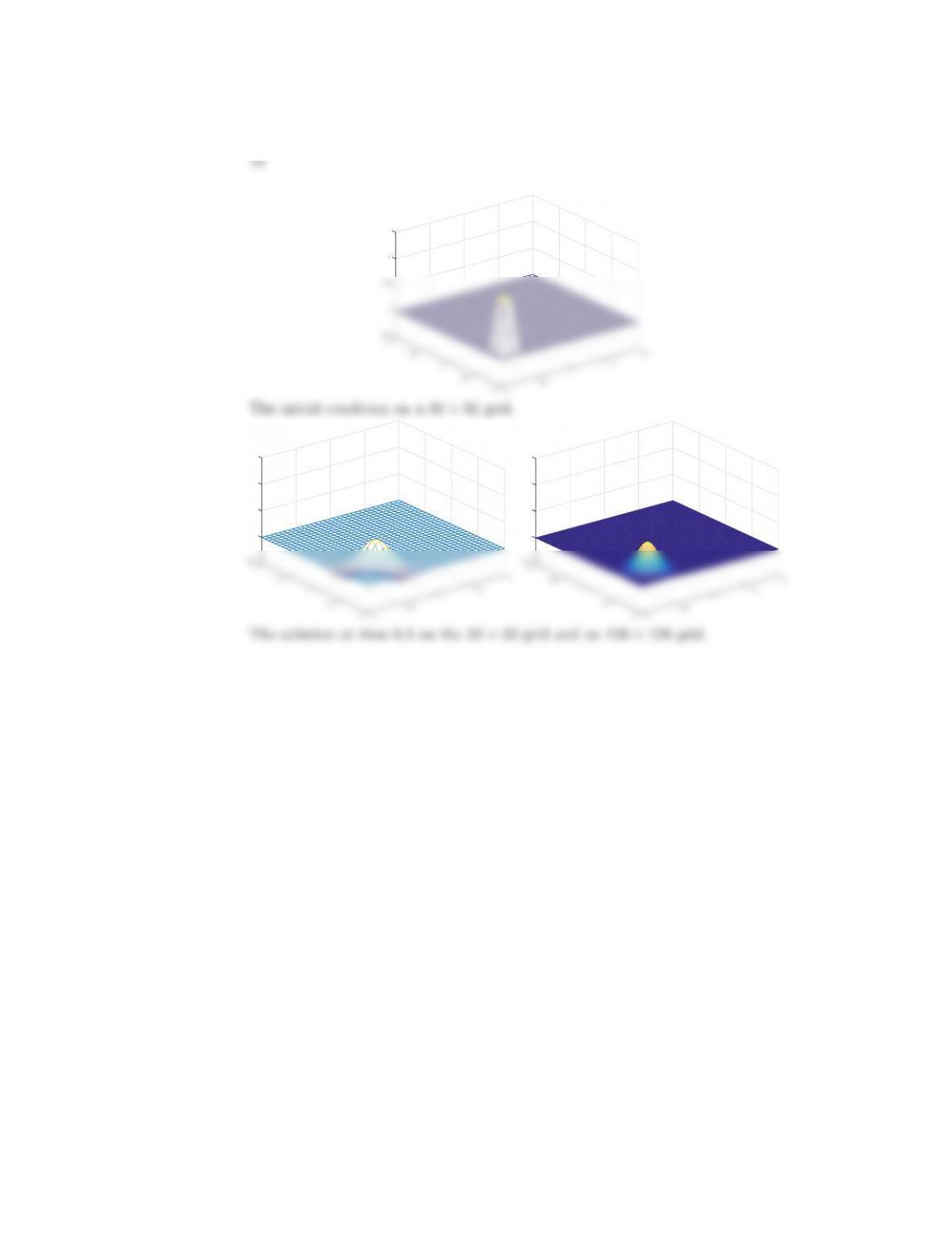
Modify the code used to solve the two-dimensional linear advection equation
(Code 2) to simulate the advection of an initially square blob with f= 1 diag-
onally across a square domain by setting u=v= 1. The dimension of the blob
is 0.2×0.2 and it is initially located near the origin. Refine the grid and show
that the solution converges by comparing the results before the blob flows out
of the domain.
Solution
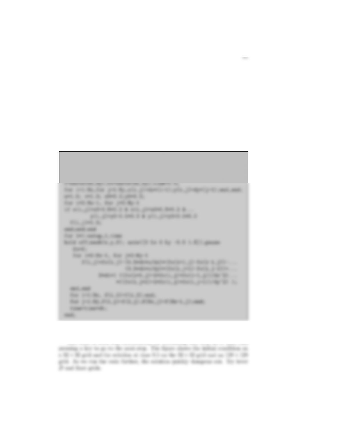
The modified code is:
% Two-dimensional unsteady diffusion by the FTCS scheme
Nx=32;Ny=32;nstep=20;D=0.025;Lx=2.0;Ly=2.0;
dx=Lx/(Nx-1); dy=Ly/(Ny-1); dt=0.02;
The code is best run interactively by advancing one step at a time and
Problem 9
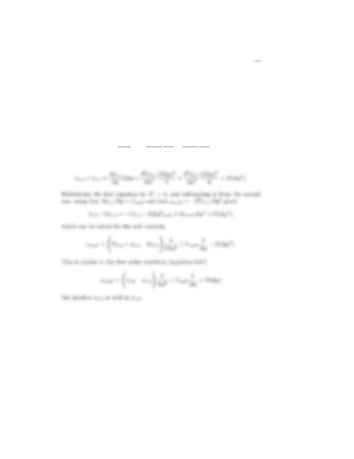
Derive a second order expression for the boundary vorticity by writing the
stream function at j= 2 and j= 3 as a Taylor series expansion around the value
at the wall (j= 1). How does the expression compare with equation (6.67).
Solution
The derivation is essentially the same as in the text. The stream function, one
mesh block away, can be expressed using a Taylor series expansion around the
boundary point:
ψi,2=ψi,1+∂ψi,1
∂y ∆y+∂2ψi,1
∂y2
∆y2
2+∂3ψi,1
∂y3
∆y3
6+O(∆y4).
Similarly, two mesh blocks away, we have
(2∆y)2
(2∆y)3
Problem 10
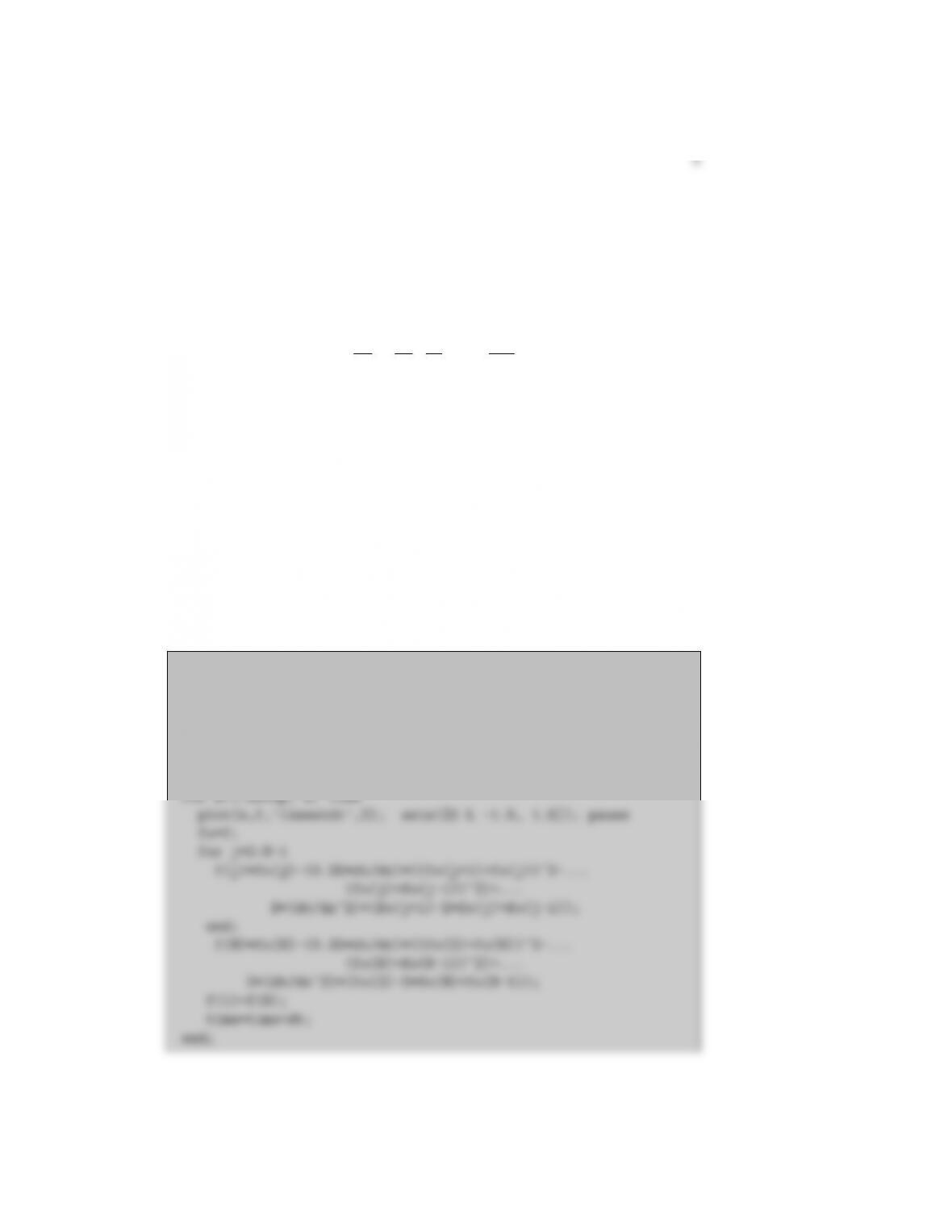
Modify the vorticity-stream function code used to simulate the two-dimensional
driven cavity problem (Code 3) to simulate the flow in a rectangular 2 ×1
channel with periodic boundaries. Set the value of the vorticity and the stream
function at the top and bottom to zero. As initial conditions place two circular
blobs with radius r= 0.25 and ω= 10 on the centerline of the channel at y= 0.5
and x= 0.6 and x= 1.4. Refine the grid to ensure that the solution converges.
Describe the evolution of the flow as the viscosity is decreased.
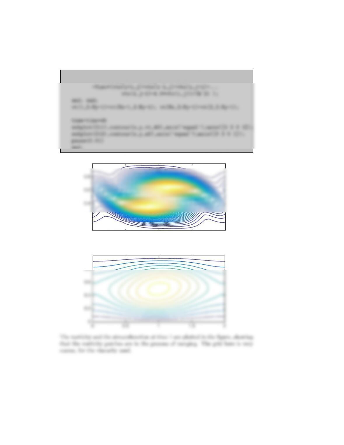
Solution
The code, modified as specified in the problem is listed below. Notice that
the viscosity here is 0.01 and that we accommodate the periodic boundary
conditions by extending the grid one grid line in the x-direction. Thus, the
grid spacing is given by h= 2.0/(Nx −2), rather than h= 2.0/(Nx −1). Here,
the 2 is the length of the domain in the x-direction.
% Problem 10 Modified Vorticity-Stream Function Code
Nx=34; Ny=17; MaxStep=200; Visc=0.01; dt=0.005; time=0.0;
MaxIt=100; Beta=1.5; MaxErr=0.001; % parameters for SOR
sf=zeros(Nx,Ny); vt=zeros(Nx,Ny); vto=zeros(Nx,Ny);
for i=2:Nx-1; for j=2:Ny-1
vt(i,j)=vt(i,j)+dt*(-0.25*((sf(i,j+1)-sf(i,j-1))*…
15
(vto(i+1,j)-vto(i-1,j))-(sf(i+1,j)-sf(i-1,j))*…
(vto(i,j+1)-vto(i,j-1)))/(h*h)…
end;
0 0.5 1 1.5 2
0
0.2
0.4
0.6
0.8
1
0 0.5 1 1.5 2
0
0.2
0.4
0.6
0.8
1
Problem 11
Derive the discrete pressure equation for a corner point. How does it compare
with the equation for an interior point, (6.91) and a point next to a straight
boundary (6.96)?
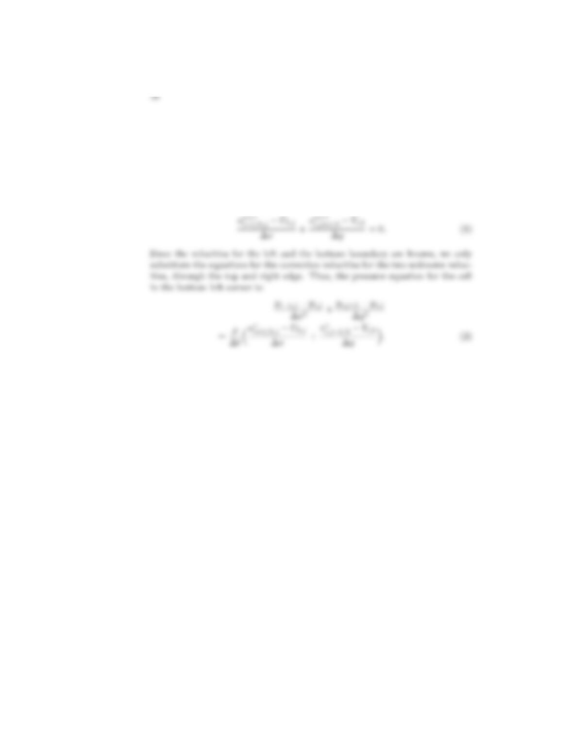
Solution
Start with the continuity equation for the cell in the lower left corner. For the
control volume around the pressure node p(2,2), it is
Problem 12
Modify the velocity-pressure code used to simulate the two-dimensional driven
cavity problem (Code 4) to simulate the mixing of a jet of fast fluid with slower
fluid. Change the size of the domain to 3 and specify an inflow velocity of 1 in
the middle third of the left boundary and an inflow velocity of 0.25 for the rest
of the boundary. For the right boundary specify a uniform outflow velocity of
0.5. Keep other parameters the same. Refine the grid and check the convergence
of the solution.
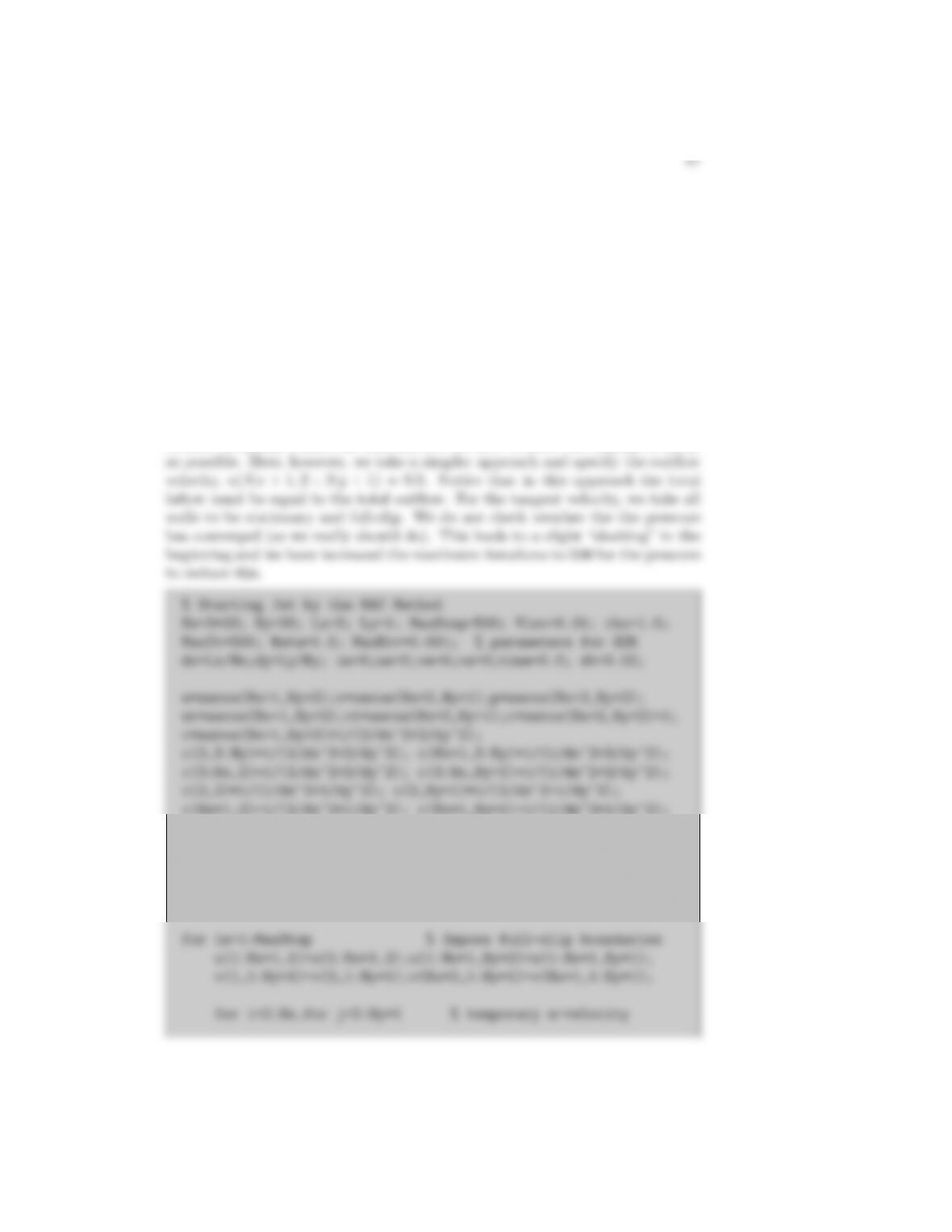
Solution
The main change is in the boundary conditions. On the left boundary we
specify the inflow by setting u(1,2 : Ny + 1) to different values depending on
whether the grid point is in the jet or not. In general we would specify “gentle”
outflow boundary conditions that allowed the flow to leave the domain as freely
Ny1=12; Ny2=23;
u(1,2:Ny+1)=0.25; u(1,Ny1:Ny2)=1.0;
u(Nx+1,2:Ny+1)=0.5;
ut=u;