Fluid Mechanics, 6th Ed. Kundu, Cohen, and Dowling
Exercise 3.1. The gradient operator in Cartesian coordinates (x, y, z) is:
∇=ex
∂ ∂
x
( )
+ey
∂ ∂
y
( )
+ez
∂ ∂
z
( )
where
ex
,
ey
, and
ez
are the unit vectors. In cylindrical polar
coordinates (R,
ϕ
, z) having the same origin, (see Figure 3.3b), coordinates and unit vectors are
related by:
R=x2+y2
,
ϕ
=tan−1y x
( )
, and z = z; and
eR=excos
ϕ
+eysin
ϕ
,
e
ϕ
=−exsin
ϕ
+eycos
ϕ
, and
ez=ez
. Determine the following in the cylindrical polar coordinate
system.
a)
∂
eR
∂ϕ
and
∂
e
ϕ∂ϕ
b) the gradient operator ∇
c) the divergence of the velocity field ∇⋅u
d) the Laplacian operator
∇ ⋅ ∇ ≡ ∇2
e) the advective acceleration term (u⋅∇)u
Solution 3.1. The Cartesian unit vectors do not depend on the coordinates so the unit vectors
from the cylindrical coordinate system can be differentiated when they are written in terms of ex,
ey, and ez.
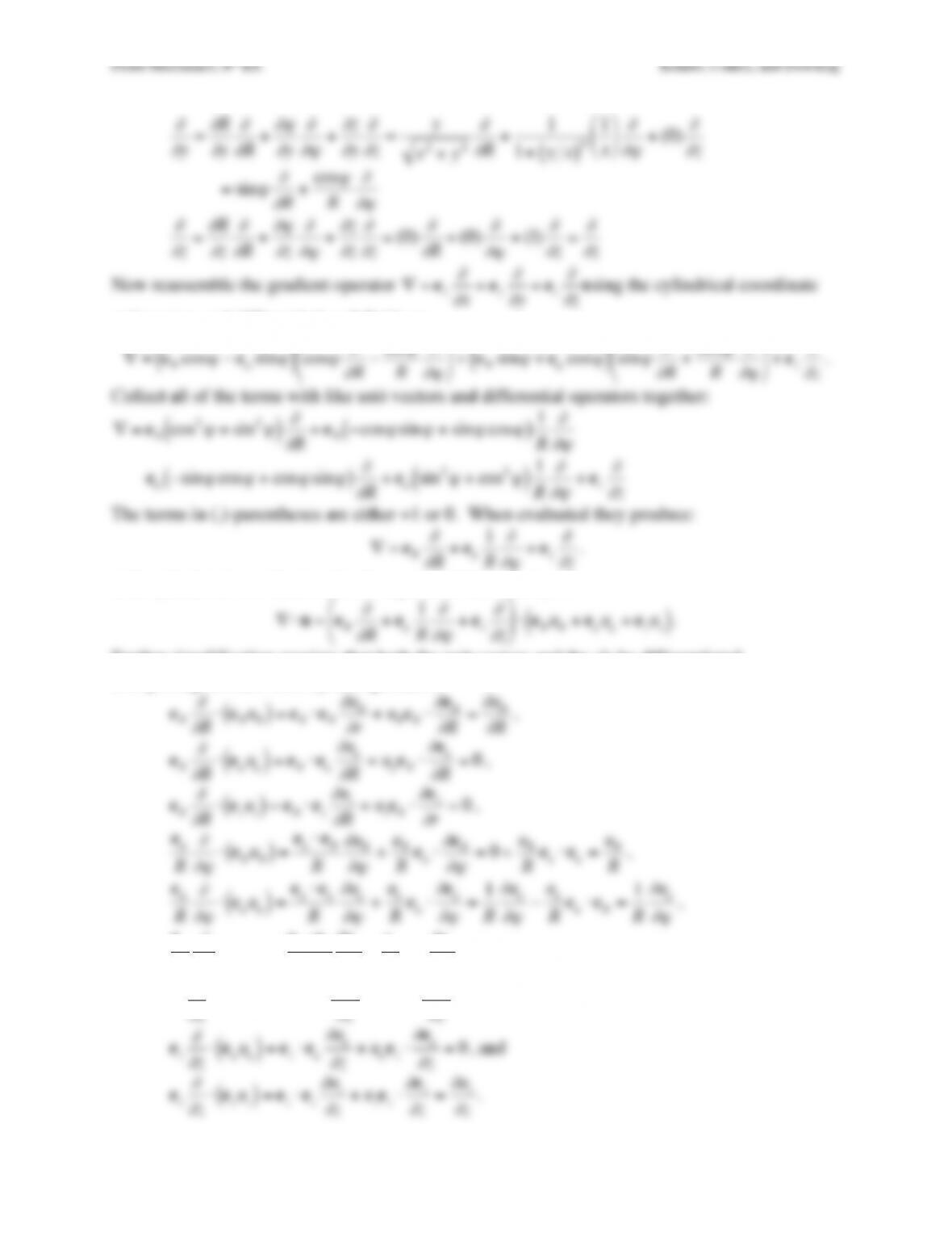
a) First work with eR, use the given unit vector definition, and proceed with straightforward
The third unit vector, ez, is the same as the Cartesian unit vector and does not depend on the
coordinates.
b) Start by constructing the expressions for ex, ey, and ez in terms of eR, e
ϕ
, and ez. This can be
done my inverting the linear system
cos
ϕ
sin
ϕ
0
−sin
ϕ
cos
ϕ
0
0 0 1
$
%
&
‘
(
)
&
*
ex
ey
ez
$
%
&
‘
(
)
&
*
=
eR
e
ϕ
ez
$
%
&
‘
(
)
&
*
to find
ex=eRcos
ϕ
−e
ϕ
sin
ϕ
,
ey=eRsin
ϕ
+e
ϕ
cos
ϕ
, and
ez=ez
(1,2,3)
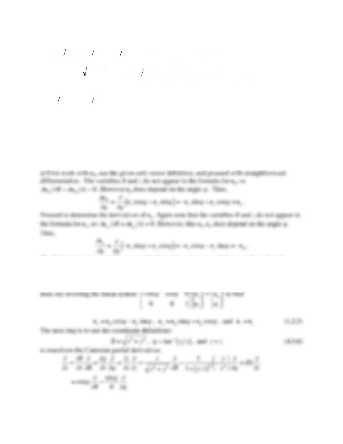
The next step is to use the coordinate definitions:
R=x2+y2
,
ϕ
=tan−1y x
( )
, and z = z (4,5,6)
Fluid Mechanics, 6th Ed. Kundu, Cohen, and Dowling
unit vectors and differentiation definitions:
∇=eRcos
ϕ
−e
ϕ
sin
ϕ
( )
cos
ϕ∂
∂
R−sin
ϕ
R
∂
∂ϕ
&
‘
(
)
*
+ +eRsin
ϕ
+e
ϕ
cos
ϕ
( )
sin
ϕ∂
∂
R+cos
ϕ
R
∂
∂ϕ
&
‘
(
)
*
+ +ez
∂
∂
z
.
Collect all of the terms with like unit vectors and differential operators together:
∇=eRcos2
ϕ
+sin2
ϕ
( )
∂
∂
R+eR−cos
ϕ
sin
ϕ
+sin
ϕ
cos
ϕ
( )
1
R
∂
∂ϕ
e
ϕ
−sin
ϕ
cos
ϕ
+cos
ϕ
sin
ϕ
( )
∂
∂
R+e
ϕ
sin2
ϕ
+cos2
ϕ
( )
1
R
∂
∂ϕ
+ez
∂
∂
z
The terms in (,)-parentheses are either +1 or 0. When evaluated they produce:
∇=eR
∂
∂
R+e
ϕ
1
R
∂
∂ϕ
+ez
∂
∂
z
.
c) In cylindrical coordinates, the divergence of the velocity is:
∇ ⋅ u=eR
∂
∂
R+e
ϕ
1
R
∂
∂ϕ
+ez
∂
∂
z
&
‘
(
)
*
+
⋅eRuR+e
ϕ
u
ϕ
+ezuz
( )
.
Further simplification requires that both the unit vectors and the u‘s be differentiated.
Completing this task term by term produces:
eR
∂
∂
R⋅eRuR
( )
=eR⋅eR
∂
uR
∂
r+uReR⋅
∂
eR
∂
R=
∂
uR
∂
R
,
e
ϕ
R
∂
∂ϕ
⋅ezuz
( )
=e
ϕ
⋅ez
R
∂
u
ϕ
∂ϕ
+uz
R
e
ϕ
⋅
∂
ez
∂ϕ
=0
ez
∂
∂
z⋅eRuR
( )
=ez⋅eR
∂
uR
∂
z+uRez⋅
∂
eR
∂
z=0
,
ez
∂
z⋅e
ϕ
u
ϕ
( )
=ez⋅e
ϕ
∂
u
∂
z+u
ϕ
ez⋅
∂
e
∂
z=0
, and
∂
uz
∂
ez
∂
uz
Fluid Mechanics, 6th Ed. Kundu, Cohen, and Dowling
Reassembling the equation produces:
∇ ⋅ u=
∂
uR
∂
R+uR
R+1
R
∂
u
ϕ
∂ϕ
+
∂
uz
∂
z
.
The 1st & 2nd terms on the right side are commonly combined to yield:
∇ ⋅ u=1
R
∂
∂
R
RuR
( )
+1
R
∂
u
ϕ
∂ϕ
+
∂
uz
∂
z
. (10)
d) The Laplacian operator is
∇2≡ ∇ ⋅ ∇
, and its form in cylindrical coordinates can be found by
evaluating the dot product. Fortunately, the results of part c) can be used via the following
replacements for the second gradient operator of the dot product:
uR↔
∂
∂
R
,
u
ϕ
↔1
R
∂
∂ϕ
, and
uz↔
∂
∂
z
. (7,8,9)
Inserting the replacements (7,8,9) into (10) produces:
∇2=1
R
∂
∂
R
R
∂
∂
R
$
%
& ‘
(
) +1
R2
∂
2
∂ϕ
2+
∂
2
∂
z2
.
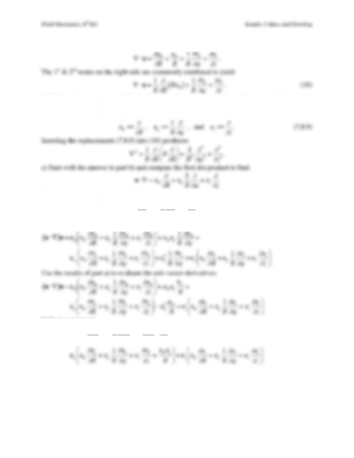
e) Start with the answer to part b) and compute the first dot product to find:
u⋅ ∇ =uR
∂
∂
R+u
ϕ
1
R
∂
∂ϕ
+uz
∂
∂
z
This is the scalar operator applied to
u=uReR+u
ϕ
e
ϕ
+uzez
to find the advective acceleration:
u⋅ ∇
( )
u=uR
∂
∂
R+u
ϕ
1
R
∂
∂ϕ
+uz
∂
∂
z
&
‘
(
)
*
+ uReR+u
ϕ
e
ϕ
+uzez
( )
.
Here the components of u and the unit vectors eR and e
ϕ
depend on the angular coordinate.
u⋅ ∇
( )
u=eRuR
∂
uR
∂
R+u
ϕ
1
R
∂
uR
∂ϕ
+uz
∂
uR
∂
z
&
‘
(
)
*
+ +uRu
ϕ
1
R
∂
eR
∂ϕ
+
e
ϕ
uR
∂
u
ϕ
∂
R+u
ϕ
1
R
∂
u
ϕ
∂ϕ
+uz
∂
u
ϕ
∂
z
!
“
#$
%
&+u
ϕ
21
R
∂
e
ϕ
∂
ϕ
+ezuR
∂
uz
∂
R+u
ϕ
1
R
∂
uz
∂ϕ
+uz
∂
uz
∂
z
!
“
#$
%
&
Use the results of part a) to evaluate the unit vector derivatives.
u⋅ ∇
( )
u=eRuR
∂
uR
∂
R+u
ϕ
1
R
∂
uR
∂ϕ
+uz
∂
uR
∂
z
&
‘
(
)
*
+ +uRu
ϕ
e
ϕ
R+
e
ϕ
uR
∂
u
ϕ
∂
R+u
ϕ
1
R
∂
u
ϕ
∂ϕ
+uz
∂
u
ϕ
∂
z
$
%
&
‘
(
) −u
ϕ
2eR
R+ezuR
∂
uz
∂
R+u
ϕ
1
R
∂
uz
∂ϕ
+uz
∂
uz
∂
z
$
%
&
‘
(
)
Collect components
u⋅ ∇
( )
u=eRuR
∂
uR
∂
R+u
ϕ
1
R
∂
uR
∂ϕ
+uz
∂
uR
∂
z−u
ϕ
2
R
‘
(
)
*
+
, +
e
ϕ
uR
∂
u
ϕ
∂
R+u
ϕ
1
R
∂
u
ϕ
∂ϕ
+uz
∂
u
ϕ
∂
z+uRu
ϕ
R
$
&
‘
) +ezuR
∂
uz
∂
R+u
ϕ
1
R
∂
uz
∂ϕ
+uz
∂
uz
∂
z
$
&
‘
)
Fluid Mechanics, 6th Ed. Kundu, Cohen, and Dowling
Exercise 3.2. Consider Cartesian coordinates (as given in Exercise no. 1) and spherical polar
coordinates (r,
θ
,
ϕ
) having the same origin (see Figure 3.3c). Here coordinates and unit vectors
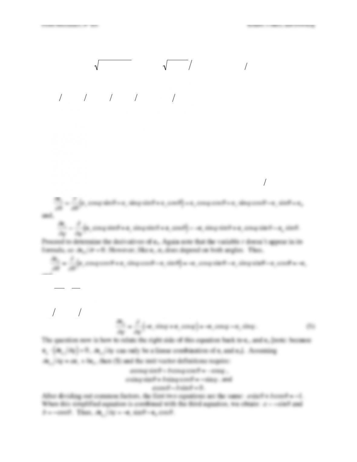
are related by:
r=x2+y2+z2
,
θ
=tan−1x2+y2z
( )
, and
ϕ
=tan−1y x
( )
; and
er=excos
ϕ
sin
θ
+eysin
ϕ
sin
θ
+ezcos
θ
,
e
θ
=excos
ϕ
cos
θ
+eysin
ϕ
cos
θ
−ezsin
θ
, and
e
ϕ
=−exsin
ϕ
+eycos
ϕ
. In the spherical polar coordinate system, determine the following items.
a)
∂
er
∂θ
,
∂
er
∂ϕ
,
∂
e
θ∂θ
,
∂
e
θ∂ϕ
, and
∂
e
ϕ∂ϕ
b) the gradient operator ∇
c) the divergence of the velocity field ∇⋅u
d) the Laplacian
∇ ⋅ ∇ ≡ ∇2
e) the advective acceleration term (u⋅∇)u
Solution 3.2. The Cartesian unit vectors do not depend on the coordinates so the unit vectors
from the spherical coordinate system can be differentiated when they are written in terms of ex,
ey, and ez.
a) First work with er, use the given unit vector definition, and proceed with straightforward
differentiation. The variable r doesn’t even appear in the formula for er, so
∂
er
∂
r=0
. However
er does depend on both angles. Thus,
∂
er
∂θ
=
∂
∂θ
excos
ϕ
sin
θ
+eysin
ϕ
sin
θ
+ezcos
θ
( )
=excos
ϕ
cos
θ
+eysin
ϕ
cos
θ
−ezsin
θ
=e
θ
and,
∂
er
∂ϕ
=
∂
∂ϕ
excos
ϕ
sin
θ
+eysin
ϕ
sin
θ
+ezcos
θ
( )
=−exsin
ϕ
sin
θ
+eycos
ϕ
sin
θ
=e
ϕ
sin
θ
.
Proceed to determine the derivatives of e
θ
. Again note that the variable r doesn’t appear in its
formula, so
∂
e
θ∂
r=0
. However, like er, e
θ
does depend on both angles. Thus,
∂
e
θ
∂θ
=
∂
∂θ
excos
ϕ
cos
θ
+eysin
ϕ
cos
θ
−ezsin
θ
( )
=−excos
ϕ
sin
θ
−eysin
ϕ
sin
θ
−ezcos
θ
=−er
and,
∂
e
θ
∂ϕ
=
∂
∂ϕ
excos
ϕ
cos
θ
+eysin
ϕ
cos
θ
−ezsin
θ
( )
=−exsin
ϕ
cos
θ
+eycos
ϕ
cos
θ
=e
ϕ
cos
θ
.
Now consider e
ϕ
and note that the variables r and
θ
don’t appear in its formula, so
∂
e
ϕ∂
r=
∂
e
ϕ∂θ
=0
. However, e
ϕ
does depend on
ϕ
. Thus,
∂
e
ϕ
∂ϕ
=
∂
∂ϕ
−exsin
ϕ
+eycos
ϕ
( )
=−excos
ϕ
−eysin
ϕ
. ($)
The question now is how to relate the right side of this equation back to er, and e
θ
[note: because
e
ϕ
⋅
∂
e
ϕ∂ϕ
( )
=0
,
∂
e
ϕ∂ϕ
can only be a linear combination of er and e
θ
]. Assuming
Fluid Mechanics, 6th Ed. Kundu, Cohen, and Dowling
b) Start by constructing the expressions for ex, ey, and ez in terms of
er
,
e
θ
, and
e
ϕ
. This can be
done my inverting the linear system
cos
ϕ
sin
θ
sin
ϕ
sin
θ
cos
θ
cos
ϕ
cos
θ
sin
ϕ
cos
θ
−sin
θ
−sin
ϕ
cos
ϕ
0
%
&
‘
(
)
*
‘
+
ex
ey
ez
%
&
‘
(
)
*
‘
+
=
er
e
θ
e
ϕ
%
&
‘
(
)
*
‘
+
to find
ex=ercos
ϕ
sin
θ
+e
θ
cos
ϕ
cos
θ
−e
ϕ
sin
ϕ
ey=ersin
ϕ
sin
θ
+e
θ
sin
ϕ
cos
θ
+e
ϕ
cos
ϕ
(1,2,3)
ez=ercos
θ
−e
θ
sin
θ
.
The next step is to use the coordinate definitions:
r=x2+y2+z2
,
θ
=tan−1x2+y2z
( )
, and
ϕ
=tan−1y x
( )
(4,5,6)
to transform the Cartesian partial derivatives.
∂
∂
x=
∂
r
∂
x
∂
∂
r+
∂θ
∂
x
∂
∂θ
+
∂ϕ
∂
x
∂
∂ϕ
=x
r
∂
∂
r+1
1+x2+y2z
( )
2
2x
2z x2+y2
∂
∂θ
−y
x2+y2
∂
∂ϕ
=cos
ϕ
sin
θ∂
∂
r+cos
ϕ
cos
θ
r
∂
∂θ
−sin
ϕ
rsin
θ
∂
∂ϕ
Fluid Mechanics, 6th Ed. Kundu, Cohen, and Dowling
The terms in (,)-parentheses are either +1 or 0. When evaluated they produce:
∇=er
∂
∂
r+e
θ
1
r
∂
∂θ
+e
ϕ
1
rsin
θ
∂
∂ϕ
.
c) In spherical coordinates, the divergence of the velocity is:
∇ ⋅ u=er
∂
∂
r+e
θ
1
r
∂
∂θ
+e
ϕ
1
rsin
θ
∂
∂ϕ
‘
(
)
*
+
,
⋅erur+e
θ
u
θ
+e
ϕ
u
ϕ
( )
.
Further simplification requires that the unit vectors and the u‘s be differentiated. Completing this
task term by term produces:
er
∂
∂
r⋅erur
( )
=er⋅er
∂
ur
∂
r+urer⋅
∂
er
∂
r=
∂
ur
∂
r
,
er
∂
∂
r⋅e
θ
u
θ
( )
=er⋅e
θ
∂
u
θ
∂
r+u
θ
er⋅
∂
e
θ
∂
r=0
,
er
∂
∂
r⋅e
ϕ
u
ϕ
( )
=er⋅e
ϕ
∂
u
ϕ
∂
r+u
ϕ
er⋅
∂
e
ϕ
∂
r=0
,
e
θ
r
∂
∂θ
⋅erur
( )
=e
θ
⋅er
r
∂
ur
∂θ
+ur
r
e
θ
⋅
∂
er
∂θ
=0+ur
r
e
θ
⋅e
θ
=ur
r
,
e
θ
r
∂
∂θ
⋅e
θ
u
θ
( )
=e
θ
⋅e
θ
r
∂
u
θ
∂θ
+u
θ
r
e
θ
⋅
∂
e
θ
∂θ
=1
r
∂
u
θ
∂θ
−u
θ
r
e
θ
⋅er=1
r
∂
u
θ
∂θ
,
e
θ
r
∂
∂θ
⋅e
ϕ
u
ϕ
( )
=e
θ
⋅e
ϕ
r
∂
u
ϕ
∂θ
+u
ϕ
r
e
θ
⋅
∂
e
ϕ
∂θ
=0
e
ϕ
rsin
θ
∂
∂ϕ
⋅erur
( )
=e
ϕ
⋅er
rsin
θ
∂
ur
∂ϕ
+ur
rsin
θ
e
ϕ
⋅
∂
er
∂ϕ
=ur
rsin
θ
e
ϕ
⋅e
ϕ
sin
θ
( )
=ur
r
,
e
ϕ
rsin
θ
∂
∂ϕ
⋅e
θ
u
θ
( )
=e
ϕ
⋅e
θ
rsin
θ
∂
u
θ
∂ϕ
+u
θ
rsin
θ
e
ϕ
⋅
∂
e
θ
∂ϕ
=u
θ
rsin
θ
e
ϕ
⋅e
ϕ
cos
θ
=u
θ
rtan
θ
,
e
ϕ
rsin
θ
∂
∂ϕ
⋅e
ϕ
u
ϕ
( )
=1
rsin
θ
e
ϕ
⋅e
ϕ
∂
u
ϕ
∂ϕ
+u
ϕ
e
ϕ
⋅
∂
e
ϕ
∂ϕ
&
‘
(
)
*
+
=1
rsin
θ
∂
u
ϕ
∂ϕ
−u
ϕ
e
ϕ
⋅ersin
θ
+e
θ
cos
θ
( )
‘
(
)
*
+
, =1
rsin
θ
∂
u
ϕ
∂ϕ
Reassembling the equation produces:
∇ ⋅ u=
∂
ur
∂
r+2ur
r+1
r
∂
u
θ
∂θ
+u
θ
rtan
θ
+1
rsin
θ
∂
u
ϕ
∂ϕ
The 1st & 2nd terms, and the 3trd and 4th terms on the right side are commonly combined to yield:
Fluid Mechanics, 6th Ed. Kundu, Cohen, and Dowling
e) Start with the answer to part b) and compute the first dot product to find:
u⋅ ∇ =ur
∂
∂
r+u
θ
1
r
∂
∂θ
+u
ϕ
1
rsin
θ
∂
∂ϕ
This is the scalar operator applied to
u=urer+u
θ
e
θ
+u
ϕ
e
ϕ
to find the advective acceleration:
u⋅ ∇
( )
u=ur
∂
∂
r+u
θ
1
r
∂
∂θ
+u
ϕ
1
rsin
θ
∂
∂ϕ
‘
(
)
*
+
, urer+u
θ
e
θ
+u
ϕ
e
ϕ
( )
.
Here the components of u and the unit vectors depend on the angular coordinates.
u⋅ ∇
( )
u=erur
∂
ur
∂
r+u
θ
1
r
∂
ur
∂θ
+u
ϕ
1
rsin
θ
∂
ur
∂ϕ
‘
(
)
*
+
, +uru
θ
1
r
∂
er
∂θ
+uru
ϕ
1
rsin
θ
∂
er
∂ϕ
+
e
θ
ur
∂
u
θ
∂
r+u
θ
1
r
∂
u
θ
∂θ
+u
ϕ
1
rsin
θ
∂
u
θ
∂ϕ
%
e
ur
u
r+u
r
u
+u
rsin
u
‘
(
* +u
θ
21
r
∂
e
θ
∂θ
+u
θ
u
ϕ
1
rsin
θ
∂
e
θ
∂ϕ
+
Collect components
u⋅ ∇
( )
u=erur
∂
ur
∂
r+u
θ
1
r
∂
ur
∂θ
+u
ϕ
1
rsin
θ
∂
ur
∂ϕ
−u
θ
2+u
ϕ
2
r
(
)
*
+
,
– +
e
θ
ur
∂
u
θ
∂
r+u
θ
1
r
∂
u
θ
∂θ
+u
ϕ
1
rsin
θ
∂
u
θ
∂ϕ
+uru
θ
r−u
ϕ
2
r
cot
θ
&
(
)
+
Fluid Mechanics, 6th Ed. Kundu, Cohen, and Dowling
Exercise 3.3. In a steady two-dimensional flow, Cartesian-component particle trajectories are
given by:
x(t)=r
ocos
γ
(t−to)+
θ
o
( )
and
y(t)=r
osin
γ
(t−to)+
θ
o
( )
where
r
o=xo
2+yo
2
and
θ
o=tan−1yoxo
( )
.
a) From these trajectories determine the Lagrangian particle velocity components u(t) = dx/dt and
v(t) = dy/dt, and convert these to Eulerian velocity components u(x,y) and v(x,y).
b) Compute Cartesian particle acceleration components, ax = d2x/dt2 and ay = d2y/dt2, and show
that they are equal to D/Dt of the Eulerian velocity components u(x,y) and v(x,y).
Solution 3.3. a) Differentiate as suggested to find:
u(t)=dx(t)
dt =−
γ
r
osin
γ
(t−to)+
θ
o
( )
and
v(t)=dy(t)
dt =
γ
r
ocos
γ
(t−to)+
θ
o
( )
.
Now use the original trajectory equations to eliminate the trig-functions:
u=−
γ
y
and
v=
γ
x
.
b) Again differentiate as suggested to find:
ax(t)=d2x(t)
dt2=−
γ
2r
ocos
γ
(t−to)+
θ
o
( )
=−
γ
2x
and
ay(t)=d2y(t)
dt2=−
γ
2r
osin
γ
(t−to)+
θ
o
( )
=−
γ
2y
.
Compute Du/Dt and Dv/Dt from the final two answers of part a):
Du
Dt =∂u
∂t+u∂u
∂x+v∂u
∂y=0−
γ
y(0) +
γ
x(−
γ
)=−
γ
2x
and
Dv
Dt =∂v
∂t+u∂v
∂x+v∂v
∂y=0−
γ
y(
γ
)+
γ
x(0) =−
γ
2y
.
The final equalities match as appropriate: ax = Du/Dt, and ay = Dv/Dt.
Fluid Mechanics, 6th Ed. Kundu, Cohen, and Dowling
Exercise 3.4. In a steady two-dimensional flow, polar coordinate particle trajectories are given
by:
r(t)=r
o
and
θ
(t)=
γ
(t−to)+
θ
o
.
a) From these trajectories determine the Lagrangian particle velocity components ur(t) = dr/dt
and,
u
θ
(t)
= rd
θ
/dt, and convert these to Eulerian velocity components ur(r,
θ
) and
u
θ
(r,
θ
)
.
b) Compute polar-coordinate particle acceleration components,
ar=d2r dt2−r d
θ
dt
( )
2
and
a
θ
=rd 2
θ
dt2+2dr dt
( )
d
θ
dt
( )
, and show that they are equal to D/Dt of the Eulerian velocity
with components ur(r,
θ
) and
u
θ
(r,
θ
)
.
Solution 3.4. a) Differentiate as suggested to find:
u
r
(t)=dr(t)
dt =0
and
u
θ
(t)=rd
θ
(t)
dt =r
γ
.
These equations are readily interpreted as Eulerian velocity components:
Fluid Mechanics, 6th Ed. Kundu, Cohen, and Dowling
Exercise 3.5. if ds = (dx, dy, dz) is an element of arc length along a streamline (Figure 3.5) and u
= (u, v, w) is the local fluid velocity vector, show that if ds is everywhere tangent to u then
dx u =dy v =dz w
.
Solution 3.5. If ds = (dx, dy, dz) and u are parallel, then they must have the same unit tangent
vector t:
t=ds
ds=(dx,dy,dz)
(dx)2+(dy)2+(dz)2=(u,v,w)
u2+v2+w2=u
u
.
The three components of this equation imply:
dx
ds=u
u
,
dy
ds=v
u
, and
dz
ds=w
u
.
But these can be rearranged to find:
ds
u=dx
u=dy
v=dz
w
.
Fluid Mechanics, 6th Ed. Kundu, Cohen, and Dowling
Exercise 3.6. For the two-dimensional steady flow having velocity components u = Sy and v =
Sx, determine the following when S is a positive real constant having units of 1/time.
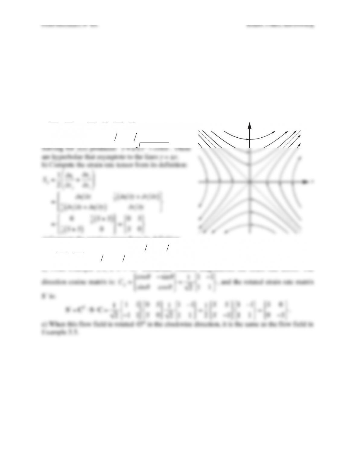
a) equations for the streamlines with a sketch of the flow pattern
b) the components of the strain rate tensor
c) the components of the rotation tensor
d) the coordinate rotation that diagonalizes the strain rate tensor, and the principal strain rates.
e) How is this flow field related to that in Example 3.5.
Solution 3.6. a) For steady streamlines in two dimensions:
dx
u=dy
v
or
dy
dx =v
u=Sx
Sy =x
y
, which implies:
ydy =xdx →y22=x22+const.
Solving for y(x) produces:
y= ± x2+const
. These
c) Compute the rotation tensor from its definition:
Rij =
∂
ui
∂
xj
−
∂
uj
∂
xi
=
0
∂
u
∂
y−
∂
v
∂
x
∂
v
∂
x−
∂
u
∂
y0
$
%
&
‘
(
) =
0S−S
S−S0
$
%
&
‘
(
) =
0 0
0 0
$
%
&
‘
(
)
d) From Example 2.4, a
θ
= 45° coordinate rotation diagonalizes the strain rate tensor. The
direction cosine matrix is:
Cij =
cos
θ
−sin
θ
sin
θ
cos
θ
$
%
‘
(
1−1
1 1
$
%
‘
(
, and the rotated strain rate matrix
y
Fluid Mechanics, 6th Ed. Kundu, Cohen, and Dowling
Exercise 3.7. At the instant shown in Figure 3.2b, the (u,v)-velocity field in Cartesian
coordinates is
u=A(y2−x2) (x2+y2)2
, and
v=−2Axy (x2+y2)2
where A is a positive
constant. Determine the equations for the streamlines by rearranging the first equality in (3.7) to
read
udy −vdx =0=
∂ψ ∂
y
( )
dy +
∂ψ ∂
x
( )
dx
and then looking for a solution in the form
ψ
(x,y) =
const.
Solution 3.7. Rearrange the two-dimensional streamline condition, dx/u = dy/v, to obtain udy –
vdx = 0 as the description of a streamline. Assume this differential equation is solved by the
function
ψ
(x,y) = const, so that (∂
ψ
/∂x)dx + (∂
ψ
/∂y)dy = 0. Comparing the two equations
requires:
u = ∂
ψ
/∂y , and v = –∂
ψ
/∂x.
Fluid Mechanics, 6th Ed. Kundu, Cohen, and Dowling
Exercise 3.8. Determine the equivalent of the first equality in (3.7) for two dimensional (r,
θ
)-
polar coordinates, and then find the equation for the streamline that passes through (ro,
θ
o) when
u = (ur, u
θ
) = (A/r, B/r) where A and B are constants.
Solution 3.8. The two-dimensional streamline condition in Cartesian coordinates is dx/u = dy/v,
and is obtained from considering the streamline-tangent vector t:
t=ds
ds=
exdx +eydy
(dx)2+(dy)2=
exu+eyv
u2+v2=u
u
.
In two-dimensional polar coordinates this becomes:
t=ds
ds=erdr +e
θ
rd
θ
(dr)2+(rd
θ
)2=erur+e
θ
u
θ
ur
2+u
θ
2=u
u
.
Equating components produces two equations:
dr
ds=ur
u
and
rd
θ
ds=u
θ
u
, or
ds
u=dr
ur
=rd
θ
u
θ
.
Thus, using the last equality and the given velocity field:
1
r
dr
d
θ
=ur
u
θ
=A r
B r =A
B→ln(r)=A
B
θ
+const.
The initial condition allows the constant to be evaluated:
ln(r
o)=A
B
θ
o+const.
, which leads to
ln r
r
o
“
#
$
%
&
‘ =A
B
θ
−
θ
o
( )
or
r=r
oexp A
B
θ
−
θ
o
( )
$
%
& ‘
(
)
.
Fluid Mechanics, 6th Ed. Kundu, Cohen, and Dowling
Exercise 3.9. Determine the streamline, path line, and streak line that pass through the origin of
coordinates at t = t´ when u = Uo +
ωξ
ocos(
ω
t) and v =
ωξ
osin(
ω
t) in two-dimensional Cartesian
coordinates where Uo is a constant horizontal velocity. Compare your results those in Example.
3.3 for
Uo→0
.
Solution 3.9. (i) For the streamline, time is a constant. Use the first equality of (3.7) to find:
dy
dx =v
u=
ωξ
osin(
ω
t)
Uo+
ωξ
ocos(
ω
t)=m(t)
,
where m is the streamline slope. Since m does not depend on the spatial coordinate, this equation
The final component equations are:
x=Uo(t−#
t )+
ξ
osin(
ω
t)−sin(
ω
#
t )
( )
and
y=–
ξ
ocos(
ω
t)−cos(
ω
%
t )
( )
.
These two parametric equations for x(t) and y(t) can be combined to eliminate some of the t–
dependence:
x−Uo(t−#
t )+
ξ
osin(
ω
#
t )
( )
2+y−
ξ
ocos(
ω
#
t )
( )
2=
ξ
o
2
,
which describes a moving circle with center located at
Uo(t−#
t )−
ξ
osin(
ω
#
t ),
ξ
ocos(
ω
#
t )
( )
.
(iii) For the streak line, use the path line results but this time evaluate the constants at t = to
instead of at t = t´ to find:
x=Uo(t−to)+
ξ
osin(
ω
t)−sin(
ω
to)
( )
and
y=–
ξ
ocos(
ω
t)−cos(
ω
to)
( )
.
Now evaluate these equations at t = t´ to produce two parametric equations for the streak line
coordinates x(to) and y(to):
x=Uo(“
t −to)+
ξ
osin(
ω
“
t )−sin(
ω
to)
( )
and
y=–
ξ
ocos(
ω
$
t )−cos(
ω
to)
( )
.
Some of the to dependence can be eliminated by combining the equations:
x−Uo(#
t −to)−
ξ
osin(
ω
#
t )
( )
2+y+
ξ
ocos(
ω
#
t )
( )
2=
ξ
o
2
,
which describes a circle with a to-dependent center located at
Uo(“
t −to)+
ξ
osin(
ω
“
t ),−
ξ
ocos(
ω
“
t )
( )
.
These results differ from those in Example 3.3 by the uniform translation velocity Uo so
they can be put into correspondence with a Galilean transformation x´ = x – Uo(t – t´).
Fluid Mechanics, 6th Ed. Kundu, Cohen, and Dowling
Exercise 3.10. Compute and compare the streamline, path line, and streak line that pass through
(1,1,0) at t = 0 for the following Cartesian velocity field u = (x, –yt, 0).
Solution 3.10. (i) For the streamline, time is a constant. Use the first equality of (3.7) to find:
dy
dx =v
u=−yt
x→dy
y=−tdx
x→ln y=−tln x+const.
, or y = const.x–t.
Evaluating at x = y = 1 and t = 0 requires the constant to be unity, so the streamline is: y = 1.
(ii) For the path line, use both components of (3.8):
dx
dt =x
and
dy
dt =−yt
,
and integrate these in time to find:
x=C1et
and
y=C2exp −t22
{ }
,
where C1 and C2 are constants. Evaluating at x = y = 1 and t = 0 requires C1 = C2 = 1. Eliminate t
from the y-equation using t = ln(x) to find the path line as:
Fluid Mechanics, 6th Ed. Kundu, Cohen, and Dowling
Exercise 3.11. Consider a time-dependent flow field in two-dimensional Cartesian coordinates
where
u=
τ
t2
,
v=xy
τ
, and
and
τ
are constant length and length time scales, respectively.
a) Use dimensional analysis to determine the functional form of the streamline through x´ at time
t´.
b) Find the equation for the streamline through x´ at time t´ and put your answer in
dimensionless form.
c) Repeat b) for the path line through x´ at time t´.
d) Repeat b) for the streak line through x´ at time t´.
Solution 3.11. a) The streamline y(x) will depend on x, t, t´, x´= (x´,y´),
, and
τ
. There are eight
parameters and two dimensions, thus there are six dimensionless groups:
y
=Ψx
,#
x
,#
y
,t
τ
,#
t
τ
%
&
‘ (
)
*
.
Here there are too many variables and parameters for dimensional analysis to be really useful.
However, this effort provides a reminder to check units throughout the remainder of the solution.
i) For the streamline, time is a constant. Use the first equality of (3.7) to find:
dy
dx =v
u=xy
τ
τ
t2→dy
y=t2
τ
2
xdx
2→ln y=t2
τ
2
x2
22+const.
The initial condition requires, x = x´ and y = y´ at t = t´, and this allows the constant to be
determined, yielding:
ln y
“
y
#
$
%
&
‘
( =(t2x2−“
t 2“
x 2)
22
τ
2
.
(ii) For the path line, use both components of (3.8):
dx
dt =
τ
t2
and
dy
dt =xy
τ
,
and integrate the first of these in time and use the initial condition to find:
x=−
τ
t+const.
or
x−#
x =−
τ
t−1−#
t −1
( )
.
Use this result for x(t) in the second equation for y(t):
dy
dt =y
τ
−
τ
1
t−1
$
t
%
&
‘ (
)
* +$
x
%
&
‘
(
)
*
or
dy
y=1
“
t −1
t+1
τ
“
x
%
&
‘ (
)
*
dt
.
The last expression can be integrated to find:
ln y
“
y
#
$
%
&
‘
( =t
“
t −1+“
x
τ
−ln t
“
t
#
$
% &
‘
( =“
x
τ
+1
“
t
#
$
% &
‘
(
(t−“
t )−ln t
“
t
#
$
% &
‘
(
or
y
“
y =t
“
t
#
$
% &
‘
(
−1
exp “
x “
t
τ
+1
#
$
% &
‘
( t
“
t −1
#
$
% &
‘
(
+
,
–
.
/
0
.
Now use the final equations for x(t) and y(t) to eliminate t. The equation for x(t) can be
rearranged to find:
“
t
t=1−(x−“
x )“
t
τ
,
so the equation for y becomes:
y
“
y =1−(x−“
x )“
t
τ
%
&
‘ (
)
*
exp “
x “
t
τ
+1
%
&
‘ (
)
* 1−(x−“
x )“
t
τ
%
&
‘ (
)
*
−1
−1
%
&
‘
‘
(
)
*
*
+
,
–
–
.
/
0
0
.
(iii) For the streak line, use the path line results but this time evaluate the integration constants at
t = to instead of at t = t´ to find:
Fluid Mechanics, 6th Ed. Kundu, Cohen, and Dowling
Fluid Mechanics, 6th Ed. Kundu, Cohen, and Dowling
Exercise 3.12. The velocity components in an unsteady plane flow are given by
u=x(1+t)
and
v=2y(2 +t)
. Determine equations for the streamlines and path lines subject to x = x0 at t = 0.
Solution 3.12. i) For the streamline, time is a constant. Use the first equality of (3.7) to find:
dy
dx =v
u=2y(2 +t)
x(1+t)→dy
y=2(1+t)
(2 +t)
dx
x→ln y=2(1+t)
(2 +t)ln x+const.
Use of the initial condition produces:
ln y0=2(1+0)
(2 +0) ln x0+const.
,
so the final answer is:
ln y
y0
“
#
$
%
&
‘ =2(1+t)
(2 +t)ln x
x0
“
#
$
%
&
‘
or
y
y0
=x
x0
“
#
$
%
&
‘
2(1+t)
(2+t)
.
(ii) For the path line, use both components of (3.8):
dx
dt =x
1+t
and
dy
dt =2y
2+t
,
and integrate the these in time to find:
ln x=ln(1+t)+const.
and
ln y=2ln(2 +t)+const.
Use the initial condition to determine the two constants, and exponentiate both equations:
x=x0(1+t)
and
y=y01+t2
( )
2
.
To determine the path line, eliminate t to find:
y=y01+(x−x0) 2x0
( )
2
.
Fluid Mechanics, 6th Ed. Kundu, Cohen, and Dowling
Exercise 3.13. Using the geometry and notation of Fig. 3.8, prove (3.9).
Solution 3.13. Before starting this problem, it is worthwhile to note that the acceleration of a
fluid particle is invariant under the specified Galilean transformation so the components of U
cannot be part of the final answer. Thus, transformation errors can be readily detected if terms
are missing in the final results or extra ones have appeared.
Figure 3.8 supports the following vector addition formula:
x=Ut+“
x
o+“
x
. Thus, the
where the final equality on each line follows from differentiating the definitions of the moving
coordinate variables given above. The time derivative requires more effort
∂
∂
t=
∂
#
x
∂
t
∂
∂
#
x +
∂
#
y
∂
t
∂
∂
#
y +
∂
#
z
∂
t
∂
∂
#
z +
∂
#
t
∂
t
∂
∂
#
t =−ex⋅U
∂
∂
#
x −ey⋅U
∂
∂
#
y −ez⋅U
∂
∂
#
z +
∂
∂
#
t
.
The first three equations imply:
∇=#
∇
and the fourth implies:
−U⋅$
∇ +
∂
∂
$
t
. The velocities will
be related by: u = U + u´. Now use these results to assemble the fluid particle acceleration
starting in the stationary coordinate system, and converting each velocity and differential
operation to the moving coordinate system.
∂
u
∂
t+u⋅ ∇
( )
u=−U⋅&
∇ +
∂
∂
&
t
‘
(
) *
+
, U+&
u
[ ]
+U+&
u
[ ]
⋅&
∇
( )
U+&
u
[ ]
=−U⋅$
∇ U+
∂
U
∂
$
t −U⋅$
∇ $
u +
∂
$
u
∂
$
t +U⋅$
∇
( )
U+$
u ⋅$
∇
( )
U+U⋅$
∇
( )
$
u +$
u ⋅$
∇
( )
$
u
Fluid Mechanics, 6th Ed. Kundu, Cohen, and Dowling
Exercise 3.14. Determine the unsteady, ∂u/∂t, and advective, (u⋅∇)u, fluid acceleration terms for
the following flow fields specified in Cartesian coordinates.
a)
u=u(y,z,t),0,0
( )
b)
u=Ω×x
where
Ω=0,0,Ωz(t)
( )
c)
u=A(t)x,−y,0
( )
d) u = (Uo + uosin(kx – Ωt), 0, 0) where Uo, uo, k and Ω are positive constants
Solution 3.14. a) Here there is only one component of the fluid velocity; thus
∂
u
∂
t=
∂ ∂
t
( )
u(y,z,t),0,0
( )
=
∂
u
∂
t,0,0
( )
, and
u⋅ ∇
[ ]
u=u(y,z,t),0,0
( )
⋅
∂ ∂
x,
∂ ∂
y,
∂ ∂
z
( )
[ ]
u(y,z,t),0,0
( )
=u(
∂ ∂
x)
[ ]
u(y,z,t),0,0
( )
=0
.
c) Again the fluid velocity has two components: (Ax, –Ay, 0), so
∂
u
∂
t=
∂ ∂
t
( )
Ax,−Ay,0
( )
=xdA
dt ,−ydA
dt ,0
$
%
& ‘
(
) =dA
dt x,−y,0
( )
, and
u⋅ ∇
[ ]
u=Ax,−Ay,0
( )
⋅
∂ ∂
x,
∂ ∂
y,
∂ ∂
z
( )
[ ]
Ax,−Ay,0
( )
u⋅ ∇
u=Uo+uosin(kx − Ωt),0,0