Unlock document.
This document is partially blurred.
Unlock all pages and 1 million more documents.
Get Access
Fluid Mechanics, 6th Ed. Kundu, Cohen, and Dowling
Exercise 2.13. Show that
δ
ij is an isotropic tensor. That is, show that
δ
'ij =
δ
ij under rotation of
the coordinate system. [Hint: Use the transformation rule (2.12) and the results of Exercise 2.10.]
Solution 2.13. Apply (2.12) to
δ
ij,
"
δ
mn =CimCjn
δ
ij =CimCin =Cmi
TCin =
δ
mn
.
where the final equality follows from the result of Exercise 2.10. Thus, the Kronecker delta is
invariant under coordinate rotations.
Fluid Mechanics, 6th Ed. Kundu, Cohen, and Dowling
Exercise 2.14. If u and v are arbitrary vectors resolved in three-dimensional Cartesian
coordinates, use the definition of vector magnitude,
a2=a⋅a
, and the Pythagorean theorem to
show that u⋅v = 0 when u and v are perpendicular.
Solution 2.14. Consider the magnitude of the sum u + v,
u+v2=(u1+v1)2+(u2+v2)2+(u3+v3)2
=u1
2+u2
2+u3
2+v1
2+v2
2+v3
2+2u1v1+2u2v2+2u3v3
=u2+v2+2u⋅v
,
which can be rewritten:
u+v2−u2−v2=2u⋅v
.
When u and v are perpendicular, the Pythagorean theorem requires the left side to be zero. Thus,
u⋅v=0
.
Fluid Mechanics, 6th Ed. Kundu, Cohen, and Dowling
Exercise 2.15. If u and v are vectors with magnitudes u and
υ
, use the finding of Exercise 2.14
to show that u⋅v = u
υ
cos
θ
where
θ
is the angle between u and v.
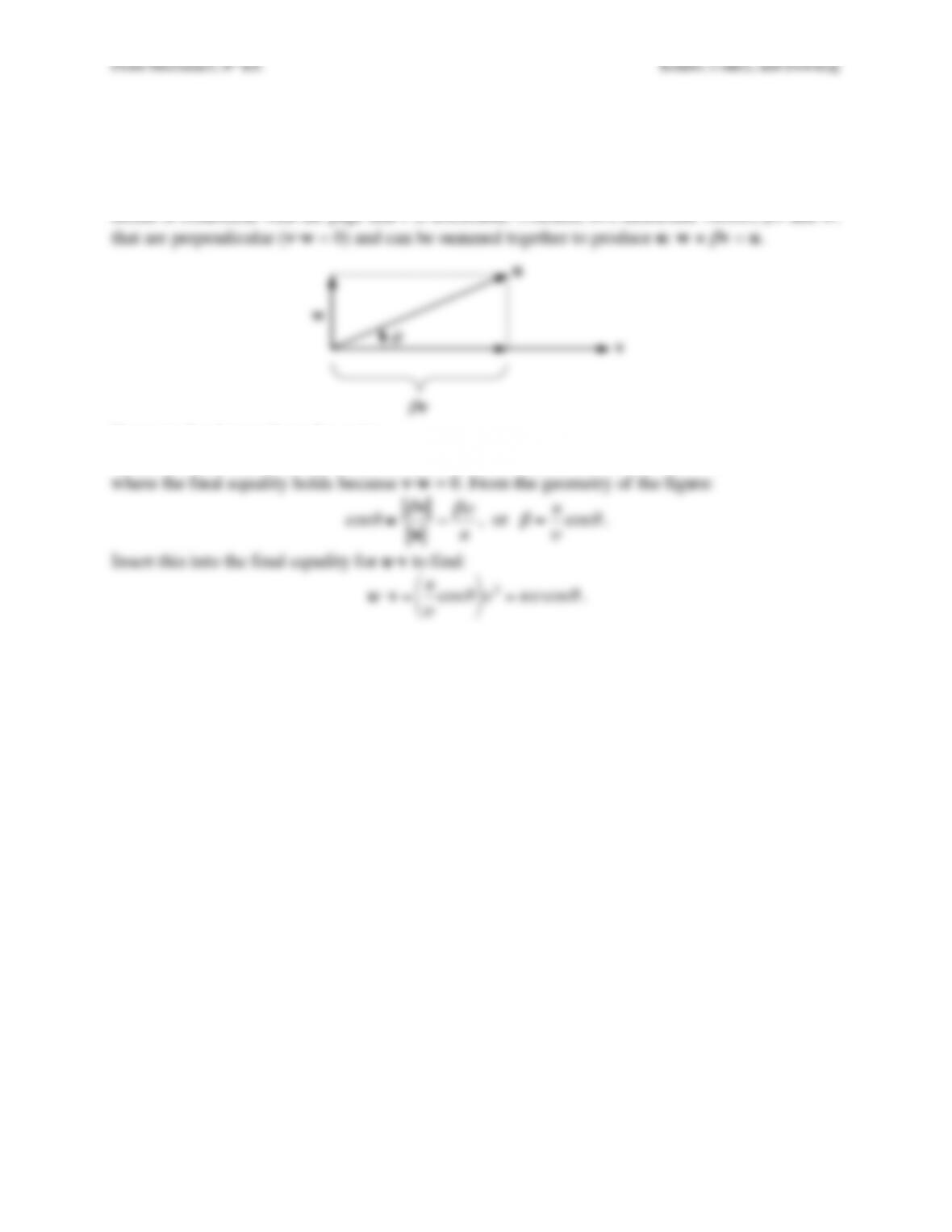
Solution 2.15. Start with two arbitrary vectors (u and v), and view them so that the plane they
define is coincident with the page and v is horizontal. Consider two additional vectors,
β
v and w,
that are perpendicular (v⋅w = 0) and can be summed together to produce u: w +
β
v = u.
Compute the dot-product of u and v:
u⋅v = (w +
β
v) ⋅v = w⋅v +
β
v⋅v =
βυ
2.
where the final equality holds because v⋅w = 0. From the geometry of the figure:
θ
u
v
β
v
w
Fluid Mechanics, 6th Ed. Kundu, Cohen, and Dowling
Exercise 2.16. Determine the components of the vector w in three-dimensional Cartesian
coordinates when w is defined by: u⋅w = 0, v⋅w = 0, and w⋅w = u2
υ
2sin2
θ
, where u and v are
known vectors with components ui and
υ
i and magnitudes u and
υ
, respectively, and
θ
is the
angle between u and v. Choose the sign(s) of the components of w so that w = e3 when u = e1
and v = e2.
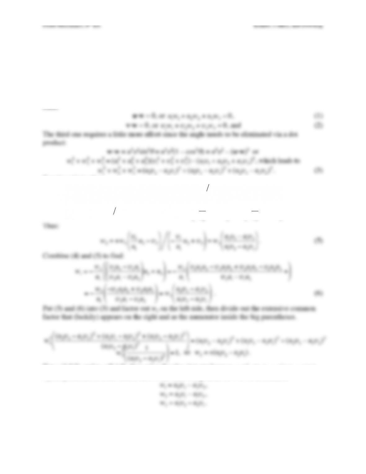
Solution 2.16. The effort here is primarily algebraic. Write the three constraints in component
form:
u⋅w = 0, or
u1w1+u2w2+u3w3=0
, (1)
Equation (1) implies:
w1=−(w2u2+w3u3)u1
(4)
Combine (2) and (4) to eliminate w1, and solve the resulting equation for w2:
−
υ
1(w2u2+w3u3)u1+
υ
2w2+
υ
3w3=0
, or
−
υ
1
u1
u2+
υ
2
$
%
&
'
(
)
w2+−
υ
1
u1
u3+
υ
3
$
%
&
'
(
)
w3=0
.
Thus:
If u = (1,0,0), and v = (0,1,0), then using the plus sign produces w3 = +1, so
w3= +(u1
υ
2−u2
υ
1)
.
Cyclic permutation of the indices allows the other components of w to be determined:
w1=u2
υ
3−u3
υ
2
,
w2=u3
υ
1−u1
υ
3
,
w3=u1
υ
2−u2
υ
1
.
Fluid Mechanics, 6th Ed. Kundu, Cohen, and Dowling
Exercise 2.17. If a is a positive constant and b is a constant vector, determine the divergence and
the curl of u = ax/x3 and u = b×(x/x2) where
x=x1
2+x2
2+x3
2≡xixi
is the length of x.
Solution 2.17. Start with the divergence calculations, and use
x=x1
2+x2
2+x3
2
to save writing.
∇ ⋅ ax
x3
$
%
& '
(
) =a
∂
∂
x1
,
∂
∂
x2
,
∂
∂
x3
$
%
&
'
(
)
⋅x1,x2,x3
x1
2+x2
2+x3
2
[ ]
3 2
$
%
&
&
'
(
)
) =a
∂
∂
x1
,
∂
∂
x2
,
∂
∂
x3
$
%
&
'
(
)
⋅x1,x2,x3
x3
$
%
& '
(
)
=a
∂
∂
x1
x1
x3
#
$
% &
'
( +
∂
∂
x2
x2
x3
#
$
% &
'
( +
∂
∂
x3
x3
x3
#
$
% &
'
(
#
%
&
( =a1
x3−3
2
x1
x52x1
( )
+1
x3−3
2
x2
x52x2
( )
+1
x3−3
2
x3
x52x3
( )
#
$
% &
'
(
Thus, the vector field ax/x3 is divergence free even though it points away from the origin
everywhere.
∇ ⋅ b×x
x2
%
&
' (
)
* =
∂
∂
x1
,
∂
∂
x2
,
∂
∂
x3
%
&
'
(
)
*
⋅b2x3−b3x2,b3x1−b
1x3,b
1x3−b2x1
x1
2+x2
2+x3
2
%
&
'
(
)
*
=
∂
∂
x1
b2x3−b3x2
x2
$
%
& '
(
) +
∂
∂
x2
b3x1−b
1x3
x2
$
%
& '
(
) +
∂
∂
x3
b
1x2−b2x1
x2
$
%
& '
(
)
$
&
'
)
This field is divergence free, too. The curl calculations produce:
∇ × ax
x3
$
%
& '
(
) =a
∂
∂
x1
,
∂
∂
x2
,
∂
∂
x3
$
%
&
'
(
) ×x1,x2,x3
x3
$
%
& '
(
) =a x3
∂
x−3
∂
x2
−x2
∂
x−3
∂
x3
,x1
∂
x−3
∂
x3
−x3
∂
x−3
∂
x1
,x2
∂
x−3
∂
x1
−x1
∂
x−3
∂
x2
$
%
&
'
(
)
=a−3
2
x3
x52x2
( )
+3
2
x2
x52x3
( )
,−3
2
x1
x52x3
( )
+3
2
x3
x52x1
( )
,−3
2
x2
x52x1
( )
+3
2
x1
x52x2
( )
#
$
% &
'
( =(0,0,0)
Fluid Mechanics, 6th Ed. Kundu, Cohen, and Dowling
Fluid Mechanics, 6th Ed. Kundu, Cohen, and Dowling
Exercise 2.18. Obtain the recipe for the gradient of a scalar function in cylindrical polar
coordinates from the integral definition (2.32).
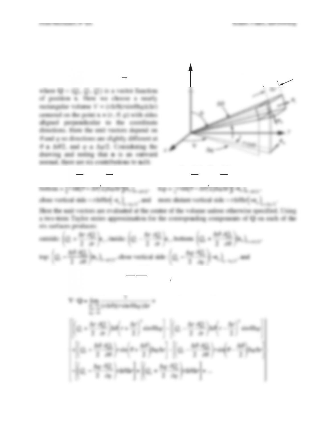
Solution 2.18. Start from the appropriate form of (2.32),
∇Ψ =lim
V→0
1
VΨndA
A
∫∫
, where Ψ is a scalar function of
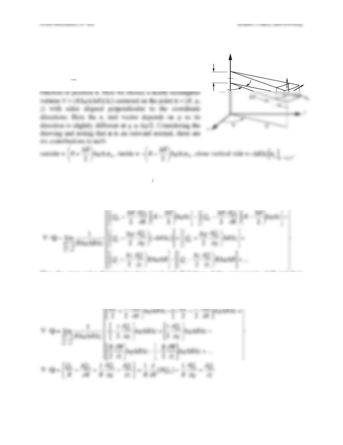
position x. Here we choose a nearly rectangular volume
and noting that n is an outward normal, there are six contributions to ndA:
outside =
R+ΔR
2
#
$
% &
'
(
Δ
ϕ
ΔzeR
, inside =
−R−ΔR
2
$
%
& '
(
)
Δ
ϕ
ΔzeR
,
close vertical side =
ΔRΔz−e
ϕ
−Δ
ϕ
2
eR
%
&
' (
)
*
, more distant vertical side =
ΔRΔze
ϕ
−Δ
ϕ
2
eR
%
&
' (
)
*
,
Δz→0
Ψ+Δz
2
∂
Ψ
∂
z
(
)
* +
,
-
ezRΔ
ϕ
ΔR
.
/
0
1
2
3
− Ψ − Δz
2
∂
Ψ
∂
z
(
)
* +
,
-
ezRΔ
ϕ
ΔR
.
/
0
1
2
3
+...
8
7
7
7
;
7
7
7
Here the mean value theorem has been used and all listings of Ψ and its derivatives above are
evaluated at the center of the volume. The largest terms inside the big {,}-brackets are
proportional to Δ
ϕ
ΔRΔz. The remaining higher order terms vanish when the limit is taken.
∇Ψ =lim
ΔR→0
Δ
ϕ
→0
Δz→0
1
RΔ
ϕ
ΔRΔz
Ψ
2
eR+R
2
∂
Ψ
∂
R
eR
(
)
*
+
,
-
Δ
ϕ
ΔRΔz− − Ψ
2
eR−R
2
∂
Ψ
∂
R
eR
(
)
*
+
,
-
Δ
ϕ
ΔRΔz+
e
ϕ
2
∂
Ψ
∂ϕ
−eR
2Ψ
(
)
*
+
,
-
Δ
ϕ
ΔRΔz+
e
ϕ
2
∂
Ψ
∂ϕ
−eR
2Ψ
(
)
*
+
,
-
Δ
ϕ
ΔRΔz+
R
2
∂
Ψ
∂
z
ez
(
)
*
+
,
-
Δ
ϕ
ΔRΔz− − R
2
∂
Ψ
∂
z
ez
(
)
*
+
,
-
Δ
ϕ
ΔRΔz+...
/
0
1
1
1
2
1
1
1
3
4
1
1
1
5
1
1
1
∇Ψ =Ψ
R
eR+
∂
Ψ
∂
R
eR+1
R
∂
Ψ
∂ϕ
e
ϕ
−Ψ
R
eR+
∂
Ψ
∂
z
ez
'
(
)
*
+
, =eR
∂
Ψ
∂
R+e
ϕ
1
R
∂
Ψ
∂ϕ
+ez
∂
Ψ
∂
z
z
e!
ez
"z
"R
"!
Fluid Mechanics, 6th Ed. Kundu, Cohen, and Dowling
Exercise 2.19. Obtain the recipe for the divergence of a vector function in cylindrical polar
coordinates from the integral definition (2.32).
Solution 2.19. Start from the appropriate form of (2.32),
∇ ⋅ Q=lim
V→0
1
Vn⋅QdA
A
∫∫
, where Q = (QR, Q
ϕ
, Qz) is a vector
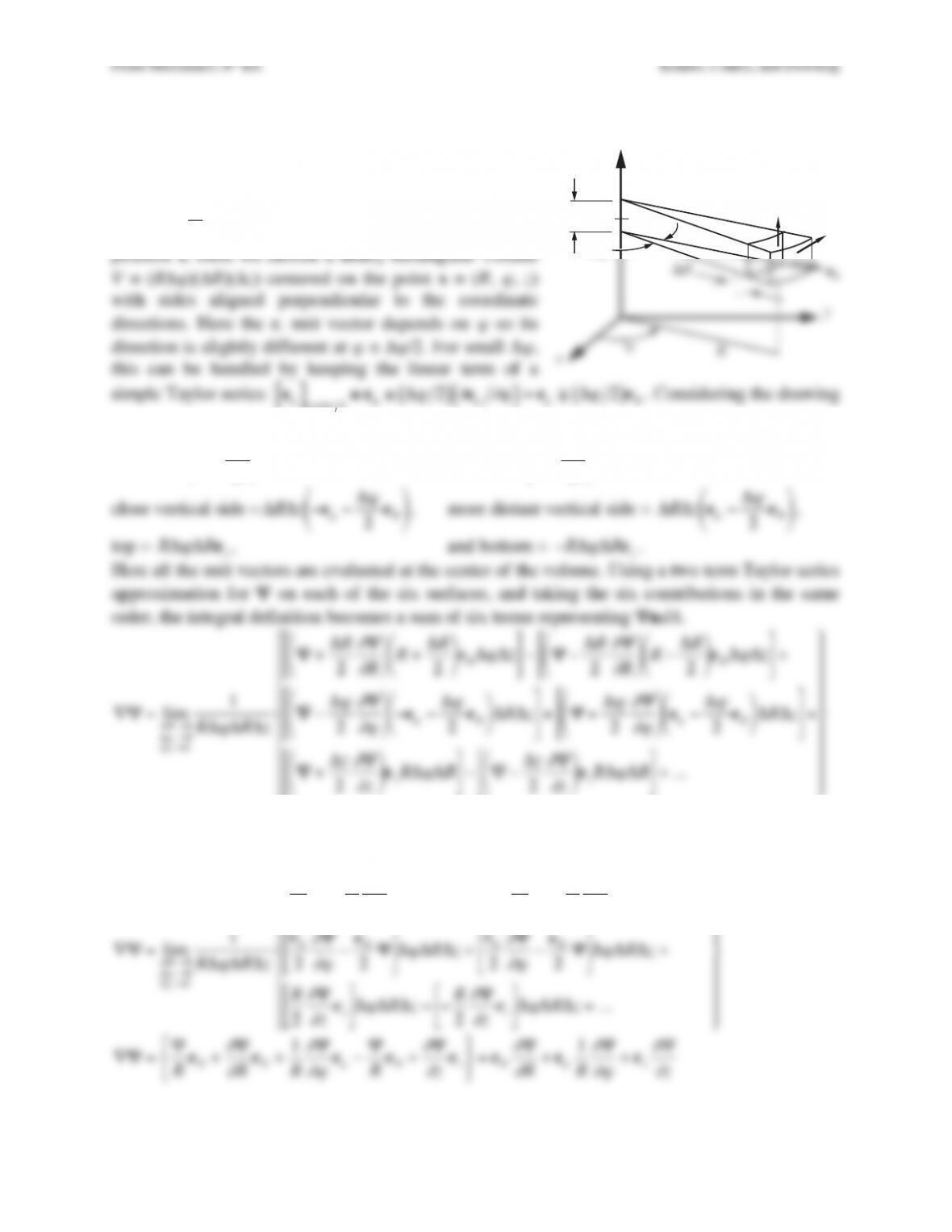
function of position x. Here we choose a nearly rectangular
more distant vertical side =
ΔRΔze
ϕ
[ ]
ϕ
+Δ
ϕ
2
, top =
RΔ
ϕ
ΔRez
, and bottom =
−RΔ
ϕ
ΔRez
.
Here the unit vectors are evaluated at the center of the volume unless otherwise specified. Using
a two-term Taylor series approximation for the components of Q on each of the six surfaces, and
taking the six contributions to
n⋅QdA
in the same order, the integral definition becomes:
∇ ⋅ Q=lim
ΔR→0
Δ
ϕ
→0
Δz→0
1
RΔ
ϕ
ΔRΔz
QR+ΔR
2
∂
QR
∂
R
(
)
* +
,
- R+ΔR
2
(
)
* +
,
-
Δ
ϕ
Δz
.
/
0
1
2
3
−QR−ΔR
2
∂
QR
∂
R
(
)
* +
,
- R−ΔR
2
(
)
* +
,
-
Δ
ϕ
Δz
.
/
0
1
2
3
+
Q
ϕ
−Δ
ϕ
2
∂
Q
ϕ
∂ϕ
(
)
*
+
,
- −ΔRΔz
( )
.
/
0
1
2
3
+Q
ϕ
+Δ
ϕ
2
∂
Q
ϕ
∂ϕ
(
)
*
+
,
-
ΔRΔz
.
/
0
1
2
3
+
Qz+Δz
2
∂
Qz
∂
z
(
)
* +
,
-
RΔ
ϕ
ΔR
.
/
0
1
2
3
−Qz−Δz
2
∂
Qz
∂
z
(
)
* +
,
-
RΔ
ϕ
ΔR
.
/
0
1
2
3
+...
5
6
7
7
7
7
8
7
7
7
7
9
:
7
7
7
7
;
7
7
7
7
Here the mean value theorem has been used and all listings of the components of Q and their
derivatives are evaluated at the center of the volume. The largest terms inside the big {,}-
brackets are proportional to Δ
ϕ
ΔRΔz. The remaining higher order terms vanish when the limit is
taken.
∇ ⋅ Q=lim
ΔR→0
Δ
ϕ
→0
Δz→0
1
RΔ
ϕ
ΔRΔz
QR
2+R
2
∂
QR
∂
R
(
)
*
+
,
-
Δ
ϕ
ΔRΔz− − QR
2−R
2
∂
QR
∂
R
(
)
*
+
,
-
Δ
ϕ
ΔRΔz+
− − 1
2
∂
Q
ϕ
∂ϕ
(
)
*
+
,
-
Δ
ϕ
ΔRΔz+1
2
∂
Q
ϕ
∂ϕ
(
)
*
+
,
-
Δ
ϕ
ΔRΔz+
R
2
∂
Ψ
∂
z
(
)
*
+
,
-
Δ
ϕ
ΔRΔz− − R
2
∂
Ψ
∂
z
(
)
*
+
,
-
Δ
ϕ
ΔRΔz+...
0
1
2
2
2
3
2
2
2
4
5
2
2
2
6
2
2
2
∇ ⋅ Q=QR
R+
∂
QR
∂
R+1
R
∂
Q
ϕ
∂ϕ
+
∂
Qz
∂
z
&
'
(
)
*
+ =1
R
∂
∂
RRQR
( )
+1
R
∂
Q
ϕ
∂ϕ
+
∂
Qz
∂
z
z
eR
e!
ez
"z
"R
"!
Fluid Mechanics, 6th Ed. Kundu, Cohen, and Dowling
Exercise 2.20. Obtain the recipe for the divergence of a vector function in spherical polar
coordinates from the integral definition (2.32).
Solution 2.20. Start from the appropriate
form of (2.32),
∇ ⋅ Q=lim
V→0
1
Vn⋅QdA
A
∫∫
,
where Q = (Qr, Q
θ
, Q
ϕ
) is a vector function
outside =
r+Δr
2
$
% &
'
(
Δ
θ
r+Δr
2
$
% &
'
(
sin
θ
Δ
ϕ
er
( )
, inside =
r−Δr
2
%
& '
(
)
Δ
θ
r−Δr
2
%
& '
(
)
sin
θ
Δ
ϕ
−er
( )
,
bottom =
rsin
θ
+Δ
θ
2
( )
Δ
ϕ
Δr
[ ]
e
θ
( )
θ
+Δ
θ
2
, top =
rsin
θ
− Δ
θ
2
( )
Δ
ϕ
Δr
[ ]
−e
θ
( )
θ
−Δ
θ
2
,
more distant vertical side :
Q
ϕ
+Δ
ϕ
2
∂
Q
ϕ
∂ϕ
%
&
'
(
)
* e
ϕ
( )
ϕ
+Δ
ϕ
2
.
Collecting and summing the six contributions to
n⋅QdA
, the integral definition becomes:
∇ ⋅ Q=lim
Δr→0
Δ
θ
→0
Δ
ϕ
→0
1
(rΔ
θ
)(rsin
θ
Δ
ϕ
)Δr×
Qr+Δr
2
∂
Qr
∂
r
*
+
, -
.
/
Δ
θ
r+Δr
2
*
+
, -
.
/
2
sin
θ
Δ
ϕ
0
1
2
3
4
5
−Qr−Δr
2
∂
Qr
∂
r
*
+
, -
.
/
Δ
θ
r−Δr
2
*
+
, -
.
/
2
sin
θ
Δ
ϕ
0
1
2
3
4
5
+Q
θ
+Δ
θ
∂
Q
θ
*
, -
/
rsin
θ
+Δ
θ
*
, -
/
Δ
ϕ
Δr
0
2
3
5
−Q
θ
−Δ
θ
∂
Q
θ
*
, -
/
rsin
θ
−Δ
θ
*
, -
/
Δ
ϕ
Δr
0
2
3
5
7
8
9
9
9
9
;
<
9
9
9
9
z
#r
Fluid Mechanics, 6th Ed. Kundu, Cohen, and Dowling
The largest terms inside the big {,}-brackets are proportional to Δ
θ
Δ
ϕ
Δr. The remaining higher
order terms vanish when the limit is taken.
∇ ⋅ Q=lim
Δr→0
Δ
θ
→0
Δ
ϕ
→0
1
(rΔ
θ
)(rsin
θ
Δ
ϕ
)Δr×
r2
∂
Qr
∂
r+2rQr
*
+
,
-
.
/
Δ
θ
sin
θ
Δ
ϕ
Δr
+sin
θ∂
Q
θ
∂θ
+cos
θ
Q
θ
*
+
,
-
.
/
rΔ
θ
Δ
ϕ
Δr
+
∂
Q
ϕ
∂ϕ
*
+
,
-
.
/
rΔ
θ
Δ
ϕ
Δr+...
0
1
2
2
2
3
2
2
2
4
5
2
2
2
6
2
2
2
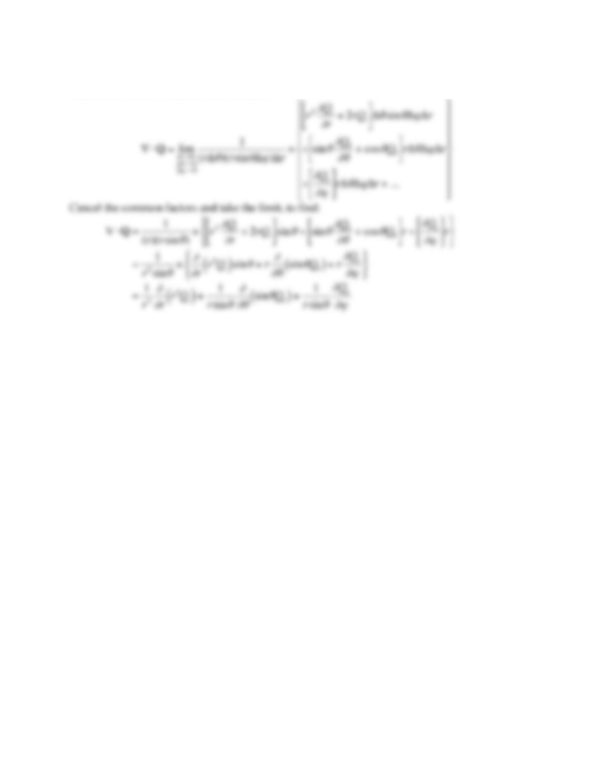
Cancel the common factors and take the limit, to find:
∇ ⋅ Q=1
(r)(rsin
θ
)×r2
∂
Qr
∂
r+2rQr
'
(
)
*
+
,
sin
θ
+sin
θ∂
Q
θ
∂θ
+cos
θ
Q
θ
'
(
)
*
+
,
r+
∂
Q
ϕ
∂ϕ
'
(
)
*
+
,
r
.
/
0
1
2
3
=1
r2sin
θ
×
∂
∂
rr2Qr
( )
sin
θ
+r
∂
∂θ
sin
θ
Q
θ
( )
+r
∂
Q
ϕ
∂ϕ
&
'
(
)
*
+
=1
r2
∂
∂
rr2Qr
( )
+1
rsin
θ
∂
∂θ
sin
θ
Q
θ
( )
+1
rsin
θ
∂
Q
ϕ
∂ϕ
Fluid Mechanics, 6th Ed. Kundu, Cohen, and Dowling
Exercise 2.21. Use the vector integral theorems to prove that
∇ ⋅ ∇ × u
( )
=0
for any twice-
differentiable vector function u regardless of the coordinate system.
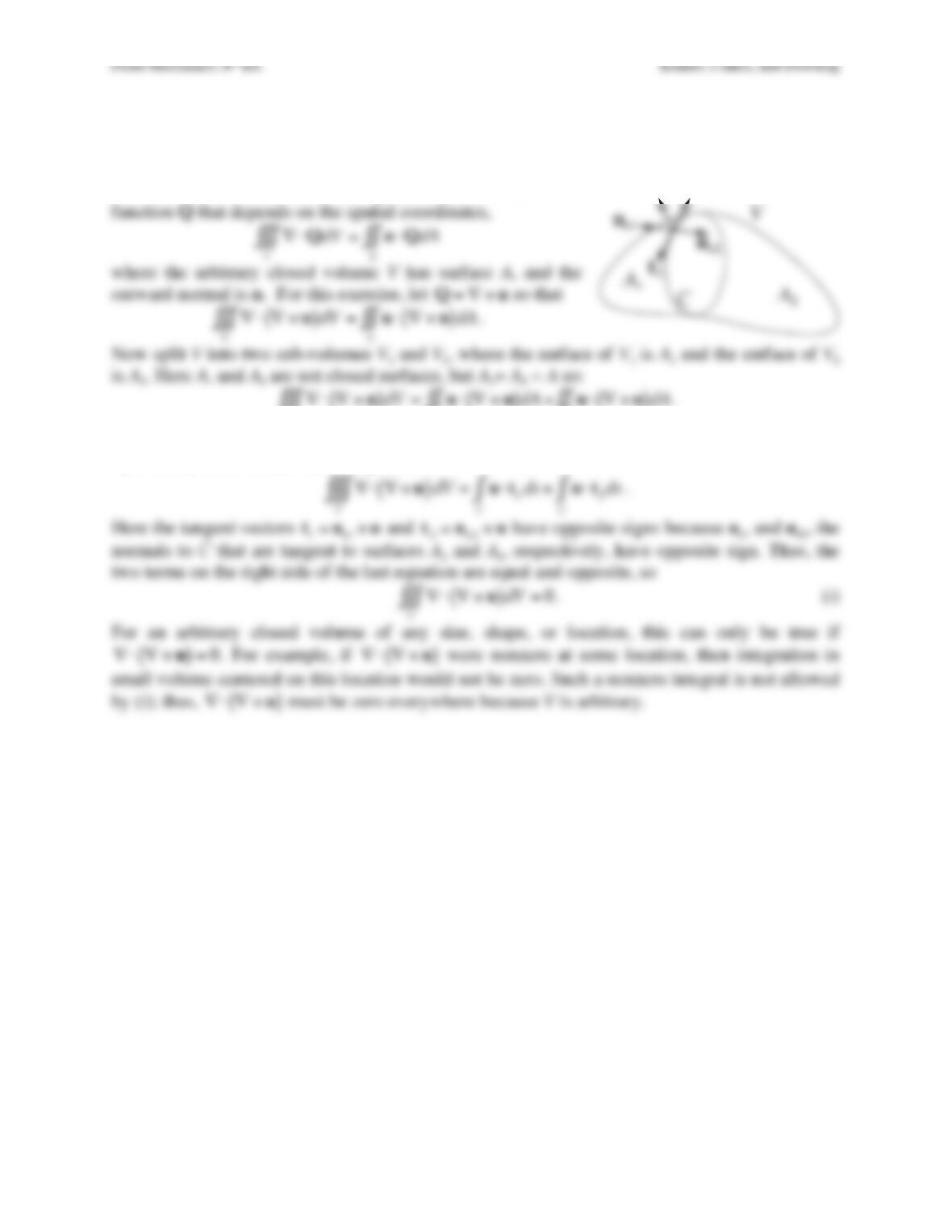
Solution 2.21. Start with the divergence theorem for a vector
function Q that depends on the spatial coordinates,
t1
nc1
n
V
Fluid Mechanics, 6th Ed. Kundu, Cohen, and Dowling
Exercise 2.22. Use Stokes’ theorem to prove that
∇ × ∇
φ
( )
=0
for any single-valued twice-
differentiable scalar
φ
regardless of the coordinate system.
Solution 2.22. From (2.34) Stokes Theorem is:
∇ × u
( )
A
∫∫ ⋅ndA =u
C
∫⋅tds
.
Let
u=∇
φ
, and note that
∇
φ
⋅tds =
∂φ ∂
s
( )
ds =d
φ
because the t vector points along the contour
C that has path increment ds. Therefore:
∇ × ∇
φ
[ ]
( )
A
∫∫ ⋅ndA =∇
φ
C
∫⋅tds =d
φ
=0
C
∫
, (ii)
where the final equality holds for integration on a closed contour of a single-valued function
φ
.
For an arbitrary surface A of any size, shape, orientation, or location, this can only be true
if
∇ × ∇
φ
( )
=0
. For example, if
∇ × ∇
φ
( )
=0
were nonzero at some location, then an area
integration in a small region centered on this location would not be zero. Such a nonzero integral
is not allowed by (ii); thus,
∇ × ∇
φ
( )
=0
must be zero everywhere because A is arbitrary.


