Fluid Mechanics, 6th Ed. Kundu, Cohen, and Dowling
Exercise 15.15. Starting from the set (15.45) with q = 0, derive (15.47) by letting station (2) be a
differential distance downstream of station (1).
Solution 15.15. The equation set (15.45) with q = 0 and the second location a differential
distance dx downstream of the first location is:
d
ρ
u
( )
=0
,
d p +
ρ
u2
( )
=−p1df
, and
d h +1
2u2
( )
=0
.
Use thermodynamic relationships to determine h in terms of p and
ρ
.
Fluid Mechanics, 6th Ed. Kundu, Cohen, and Dowling
Exercise 15.16. Starting from the set (15.45) with f = 0, derive (15.48) by letting station (2) be a
differential distance downstream of station (1).
Solution 15.16. The equation set (15.45) with f = 0 and the second location a differential
distance dx downstream of the first location is:
d
ρ
u
( )
=0
,
d p +
ρ
u2
( )
=0
, and
d h +1
2u2
( )
=h1dq
.
Use h = cpT, expand all three equations, and use the perfect gas law (p =
ρ
RT) to find:
ρ
du +ud
ρ
=0
,
dp +
ρ
du2+u2d
ρ
=0
,
cpdT +1
2du2=h1dq
, and
dp =
ρ
RdT +RTd
ρ
.
Solve the first equation for
d
ρ
=−
ρ
du u
, and eliminate d
ρ
from the second and last equations to
reach:
dp +
ρ
du2−
ρ
udu =dp +
ρ
udu =0
, and
dp
p=dT
T−du
u
,
where the final form of the last equation is obtained by dividing by p or
ρ
RT. Solve the first of
these for dp = –
ρ
udu, and use this to eliminate dp from the second:
−
ρ
udu
p=−
γ
c2udu =dT
T−du
u
.
where
γ
p/
ρ
= c2, where c = sound speed, has been used for the first equality. Solve for udu and
use M = u/c:
−
γ
c2udu +du
u=−
γ
M2−1
( )
du
u=dT
T
, or
udu =1
2du2=−u2dT
T
γ
M2−1
( )
.
Substitute this into the differential energy equation (the one that involves cp) and use h1 = cpT1,
cpdT −u2dT
T
γ
M2−1
( )
=h1dq =cpT
1dq
.
Divide this equation by
γ
R, recognize the factor of M2, and use
cp
γ
R=1
γ
−1
( )
:
cp
γ
RdT −u2dT
γ
RT
γ
M2−1
( )
=cpT
1
γ
Rdq
, or
1
γ
−1−M2
γ
M2−1
( )
$
%
&
&
‘
(
)
)
dT =1
γ
−1T
1dq
.
Solve for dT/T1.
1−(
γ
−1)M2
γ
M2−1
( )
$
%
&
&
‘
(
)
)
dT
T
1
=−1+M2
γ
M2−1
$
%
&
‘
(
) dT
T
1
=dq
, or
dT
T
1
=1−
γ
M2
1−M2dq
.
The final equation is the first part of (15.48) which shows that heat addition leads to cooling of
the gas when
1
γ
<M<1.
To reach the second part of (15.48), multiply the result for dT/T1 by
T1 and substitute this into the differential energy equation:
cpdT +udu =cpT
1
1−
γ
M2
1−M2dq
“
#
$%
&
‘+udu =h1dq
.
Recognize h1 = cpT1, and collect terms:
udu
h1
=1−1−
γ
M2
1−M2
$
%
&
‘
(
)
dq =(
γ
−1)M2
1−M2dq
.
This is the second equation of (15.48).
Fluid Mechanics, 6th Ed. Kundu, Cohen, and Dowling
Exercise 15.17. For flow of a perfect gas entering a constant area duct at Mach number M1,
calculate the maximum admissible values of f and q for the same mass flow rate. Case (a) f = 0;
case (b) q = 0.
Solution 15.17. From Section 15.6,
M2
M1
=1+
γ
M2
2
1+
γ
M1
2−f
1+(
γ
−1) 2
( )
M1
2+q
1+(
γ
−1) 2
( )
M2
2
$
%
&
‘
(
)
1 2
.
For maximum values of f or q, the flow is choked at the duct exit so M2 = 1.
a) f = 0; set M2 = 1 to find:
Fluid Mechanics, 6th Ed. Kundu, Cohen, and Dowling
Exercise 15.18. Show that the accelerating portion of the piston trajectory (0 ≤ xp(t) ≤ cot1)
shown in Figure 15.18 is:
xp(t)=
γ
+1
γ
−1
“
#
$%
&
‘cot1
t
t1
“
#
$%
&
‘
2
γ
+1
−2cot
γ
−1
for
1≤t
t1
≤2
γ
+1
“
#
$%
&
‘
1+
γ
1−
γ
.
Solution 15.18. As described in Example 15.7, the C+ characteristics emanate from the origin
during the time that the piston is accelerating. And, as described in the solution to this same
example, the C– characteristics originate on the x-axis where u = 0 and c = co, so the I– invariant
implies:
I−=u(x,t)−2c(x,t)
γ
−1=u(x, 0) −2c(x, 0)
γ
−1=−2co
γ
−1
or
c=co+
γ
−1
2
u
.
Thus, on the C+ characteristics,
2
γ
xp(t)=
γ
+1
γ
−1
t1
γ
−1
γ
+1
“
$%
‘cot1
t
“
$%
‘
γ
+1
−2cot
for
1≤t
≤2
“
$%
‘
1−
γ
,
Fluid Mechanics, 6th Ed. Kundu, Cohen, and Dowling
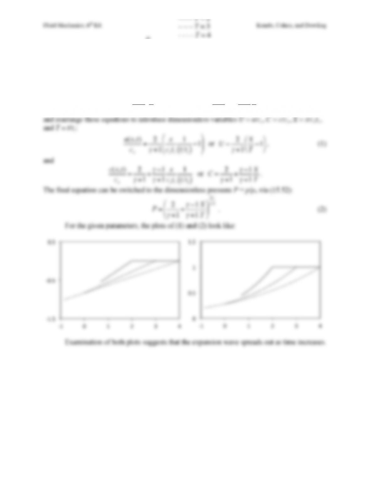
Exercise 15.19. For the flow conditions of Figure 15.18, plot u/co and p/po as functions of x/cot1
for xp(t) < x < cot at t/t1 = 2, 3, and 4 for
γ
= 1.4, where co and po are the sound speed and pressure
of the quiescent gas upstream of any disturbance from the moving piston. Does the progression
of these waveforms indicate expansion wave steepening or spreading as t increases?
Solution 15.19. Start from the results of Example 15.7,
u(x,t)=2
γ
+1
x
t−co
“
#
$%
&
‘
and
c(x,t)=2
γ
+1
co+
γ
−1
γ
+1
x
t
,
and rearrange these equations to introduce dimensionless variables U = u/co, C = c/co, X = x/cot1,
X
–––– T = 2
– – – T = 3
– – – – T = 4
P
X
–––– T = 2
– – – T = 3
– – – – T = 4
Fluid Mechanics, 6th Ed. Kundu, Cohen, and Dowling
Exercise 15.20. Consider the field properties in Figure 15.19 before the formation of the shock
wave.
a) Using the piston trajectory from Exercise 15.18, show that the time at which the piston reaches
speed co is
−t1(
γ
+1) 2
( )
(1+
γ
) (1−
γ
)
= –0.3349t1 for
γ
= 1.4.
b) Plot u/co and p/po as functions of x/cot1 for xp(t) < x < cot1 at: t/t1 = –1/3, –1/6, and –1/25 for
γ
= 1.4, where co and po are the sound speed and pressure of the quiescent gas upstream of any
disturbance from the moving piston. Does the progression of these waveforms indicate
compression wave steepening or spreading as
t→0
?
Solution 15.20. a) For the situation shown in Figure 15.19, the initial piston location is –cot1, so
the sign of xp must be changed in the formula given in Exercise 15.18, and the piston starts
moving at t = –t1, where t1 is presumed to be positive. Thus, the starting point for this Exercise
is:
xp(t)=−
γ
+1
γ
−1
“
#
$%
&
‘cot1
t
−t1
“
#
$%
&
‘
2
γ
+1
+2cot1
γ
−1
t
−t1
“
#
$%
&
‘
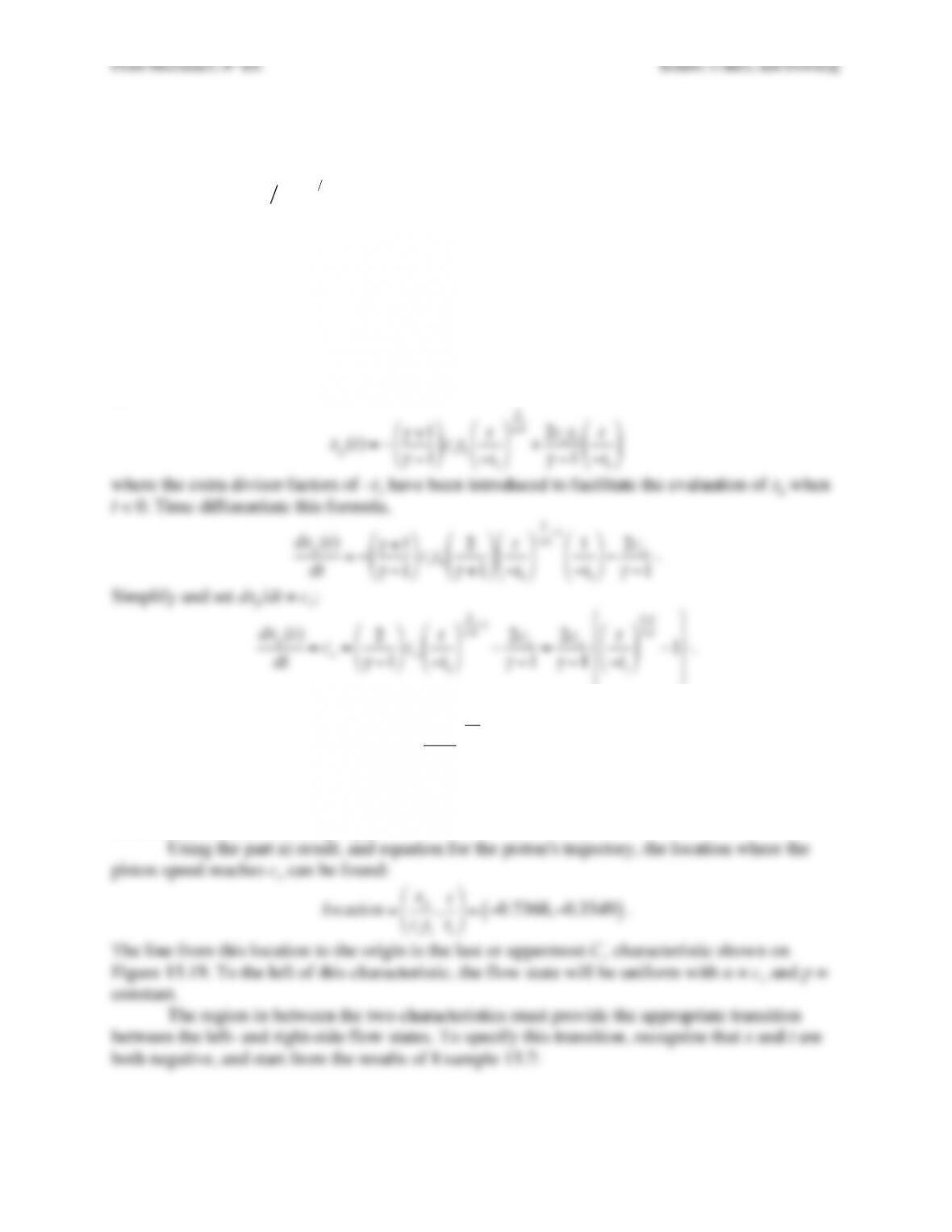
where the extra divisor factors of –t1 have been introduced to facilitate the evaluation of xp when
t < 0. Time differentiate this formula,
dxp(t)
dt =−
γ
+1
γ
−1
“
#
$%
&
‘cot1
2
γ
+1
“
#
$%
&
‘t
−t1
“
#
$%
&
‘
2
γ
+1−11
−t1
“
#
$%
&
‘−2co
γ
−1
.
Simplify and set dxp/dt = co:
dxp(t)
dt =co=2
γ
−1
“
#
$%
&
‘co
t
−t1
“
#
$%
&
‘
2
γ
+1−1
−2co
γ
−1=2co
γ
−1
t
−t1
“
#
$%
&
‘
1−
γ
1+
γ
−1
(
)
*
+
*
,
–
*
.
*
.
Divide out the common factor of co and solve for t:
t=−t1
γ
+1
2
“
#
$%
&
‘
1+
γ
1−
γ
= –0.3349t1,
where the numerical value applies when
γ
= 1.4.
b) The first or lowest C+ characteristic shown on Figure 15.19 has a slope unity. To the right of
this characteristic, u = 0 and p = po.
Using the part a) result, and equation for the piston’s trajectory, the location where the
Fluid Mechanics, 6th Ed. Kundu, Cohen, and Dowling
u(x,t)=2
γ
+1
x
t−co
“
#
$%
&
‘
and
c(x,t)=2
γ
+1
co+
γ
−1
γ
+1
x
t
.
Rearrange and introduce dimensionless variables U = u/co, C = c/co, X = x/cot1, and T = t/t1.
u(x,t)
co
=2
γ
+1
x
cot1
1
t t1
( )
−1
“
#
$
$
%
&
‘
‘
or
U=2
γ
+1
X
T−1
“
#
$%
&
‘
(1)
c(x,t)
co
=2
γ
+1+
γ
−1
γ
+1
x
cot1
1
t t1
( )
or
C=2
γ
+1+
γ
−1
γ
+1
X
T
.
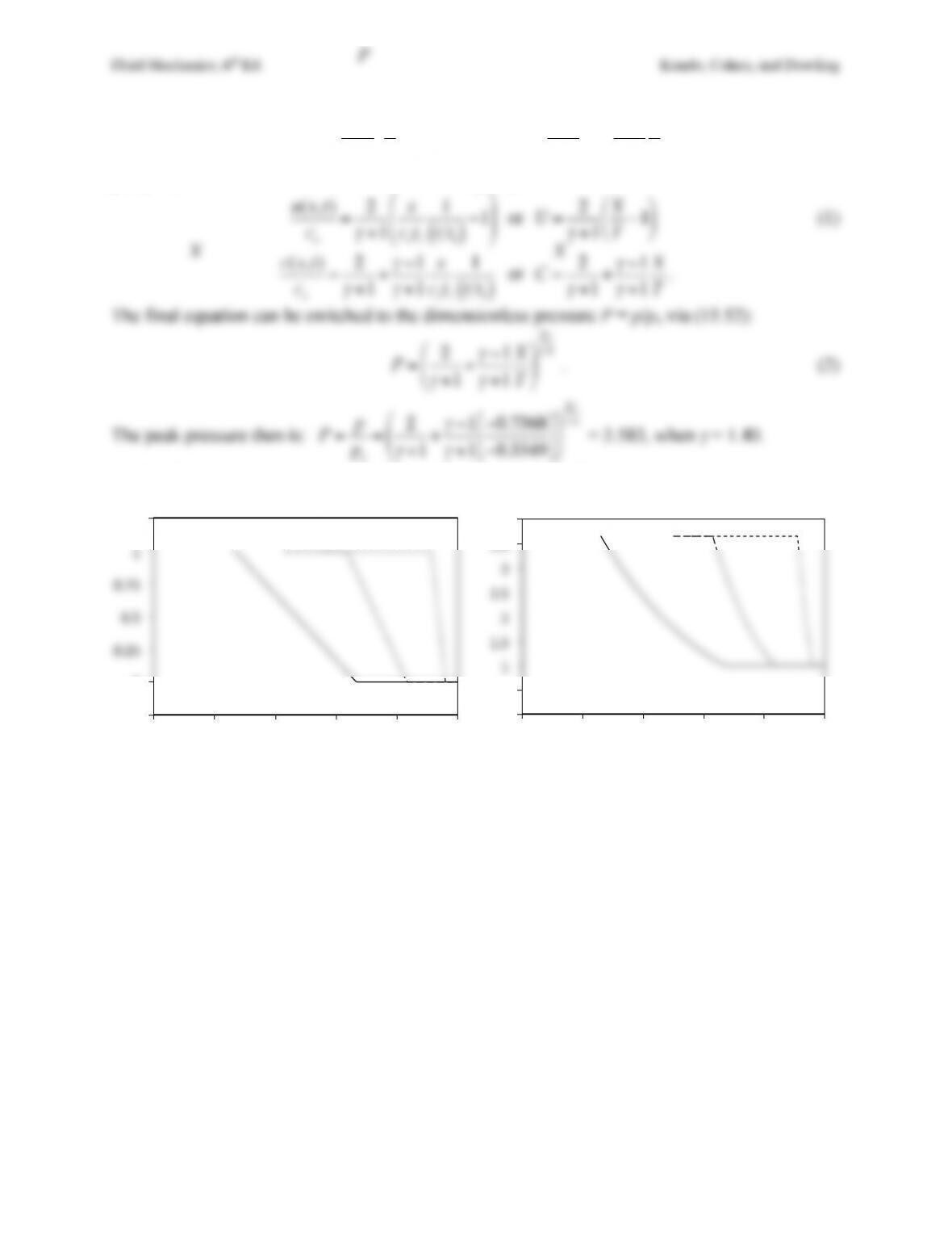
The final equation can be switched to the dimensionless pressure P = p/po via (15.52):
P=2
γ
+1+
γ
−1
γ
+1
X
T
“
#
$%
&
‘
2
γ
γ
−1
. (2)
The peak pressure then is:
P=p
po
=2
γ
+1+
γ
−1
γ
+1
−0.7368
−0.3349
“
#
$%
&
‘
(
)
*+
,
–
2
γ
γ
−1
= 3.583, when
γ
= 1.40.
For the given parameters, the plots of (1) and (2) look like:
Examination of both plots suggests that the compression wave steepens as time increases.
!0.25&
0&
0.25&
0.5&
0.75&
1&
1.25&
!1& !0.8& !0.6& !0.4& !0.2& 0&
0″
0.5″
1″
1.5″
2″
2.5″
3″
3.5″
4″
)1″ )0.8″ )0.6″ )0.4″ )0.2″ 0″
X
–––– T = 2
– – – T = 3
– – – – T = 4
P
X
–––– T = 2
– – – T = 3
– – – – T = 4
Fluid Mechanics, 6th Ed. Kundu, Cohen, and Dowling
Exercise 15.21. For the flow conditions of Figure 15.19, assume the flow speed downstream of
the shock wave is co and determine the shock Mach number, its x–t location, and the pressure,
temperature and density ratios across the shock. Are these results well matched to the isentropic
compression that occurred for t < 0? What additional adjustment is needed?
Solution 15.21. The shock wave first forms at the origin in Figure 15.19, and the velocity
difference across the shock wave is co. This is enough to determine the shock Mach number.
Start with the normal shock velocity ratio condition (15.41) for a stationary normal shock wave:
u1
u2
=(
γ
+1)M1
2
(
γ
−1)M1
2+2
. (15.41)
When the situation in Figure 15.19 is subject to a Galilean transformation that creates a shock-
p2
p1
=1+2
γ
γ
+1M1
2−1
“
#$
%=3.473
, (3.583)
ρ
2
ρ
1
=(
γ
+1)M1
2
(
γ
−1)M1
2+2=2.305
, and (2.488)
T2
T
1
=1+2(
γ
−1)
(
γ
+1)2
γ
M1
2+1
M1
2M1
2−1
( )
=1.506
. (1.440)
Interestingly, these ratios are all slightly different than the ratios produced by the
isentropic compression that occurs before the shock wave forms at t = 0 (provided in parenthesis
at the right). [These numbers are obtained from the solution of Exercise 15.20]. Thus, there will
be an adjustment region near the origin in Fig. 15.19 that will allow the pressure behind the
shock to equilibrate with the adiabatically compressed gas that is between the piston and the
shock wave. The net effect of this adjustment will be to shift the shock wave location slightly
farther ahead – in the positive x-direction – compared to what is calculated above because the
adiabatic compression reaches a higher pressure.
Fluid Mechanics, 6th Ed. Kundu, Cohen, and Dowling
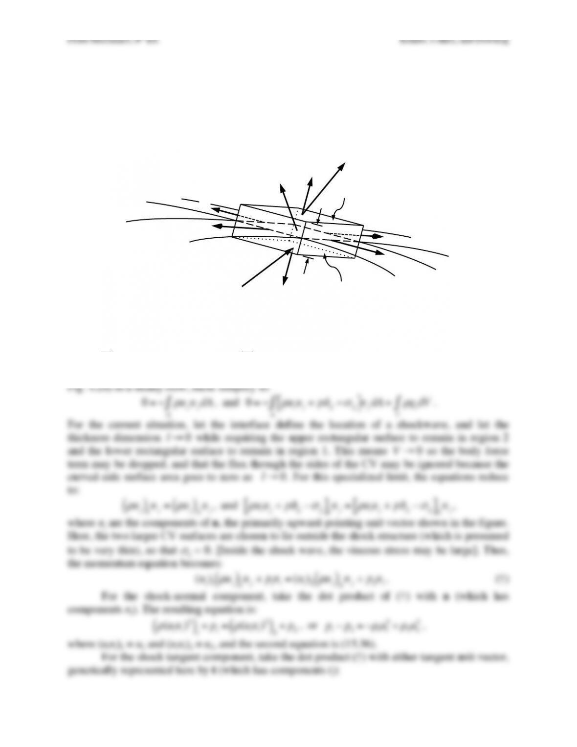
Exercise 15.22. Write momentum conservation for the volume of the small rectangular control
volume shown in Figure 4.20 where the interface is a shock with flow from side 1 to side 2. Let
the two end faces approach each other as the shock thickness → 0 and assume viscous stresses
may be neglected on these end faces (outside the structure). Show that the n component of
momentum conservation yields (15.36) and the t component gives u⋅t is conserved or v is
continuous across the shock.
Solution 15.22. For a stationary control volume V containing only fluid particles bounded by a
surface A, conservation of mass and momentum may be written:
d
dt
ρ
V
∫dV =−
ρ
uj
A
∫njdA
, and
d
dt
ρ
ui
V
∫dV =−
ρ
uiuj+p
δ
ij −
σ
ij
[ ]
A
∫njdA +
ρ
gidV
V
∫
.
When applied to a small rectangular control volume like that shown above (a reproduction of
Fig. 4.20) in a steady flow, these simplify to:
(2)!
(1)!
l!
+n!
–n!
u2!
u1!
us!
dA!
dA!

Fluid Mechanics, 6th Ed. Kundu, Cohen, and Dowling

Fluid Mechanics, 6th Ed. Kundu, Cohen, and Dowling
Exercise 15.23. A wedge has a half-angle of 50°. Moving through air, can it ever have an
attached shock? What if the half-angle were 40°? [Hint: The argument is based entirely on
Figure 15.22.]
Fluid Mechanics, 6th Ed. Kundu, Cohen, and Dowling
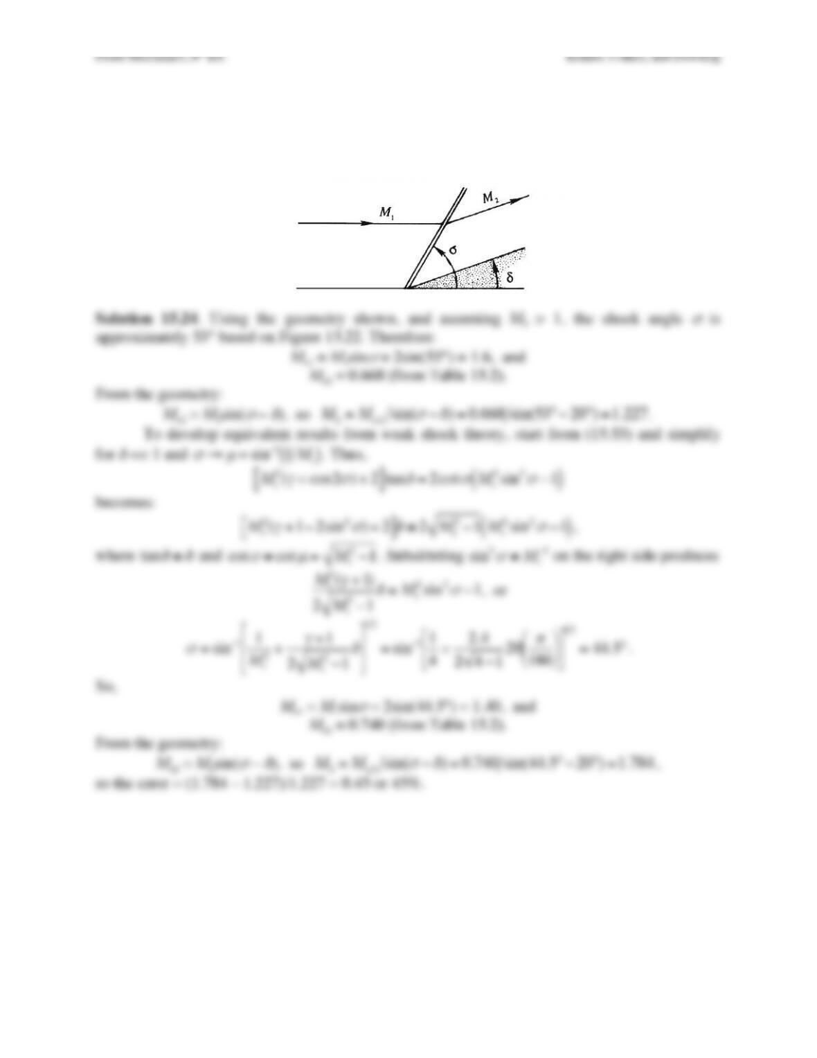
Exercise 15.24. Air at standard atmospheric conditions is flowing over a surface at a Mach
number of M1 = 2. At a downstream location, the surface takes a sharp inward turn by an angle of
20°. Find the wave angle σ and the downstream Mach number. Repeat the calculation by using
the weak shock assumption and determine its accuracy by comparison with the first method.
Solution 15.24. Using the geometry shown, and assuming M2 > 1, the shock angle
σ
is

Fluid Mechanics, 6th Ed. Kundu, Cohen, and Dowling
Exercise 15.25. A flat plate is inclined at 10° to an airstream moving at M∞ = 2. If the chord
length is b = 3 m, find the lift and wave drag per unit span.
Fluid Mechanics, 6th Ed. Kundu, Cohen, and Dowling
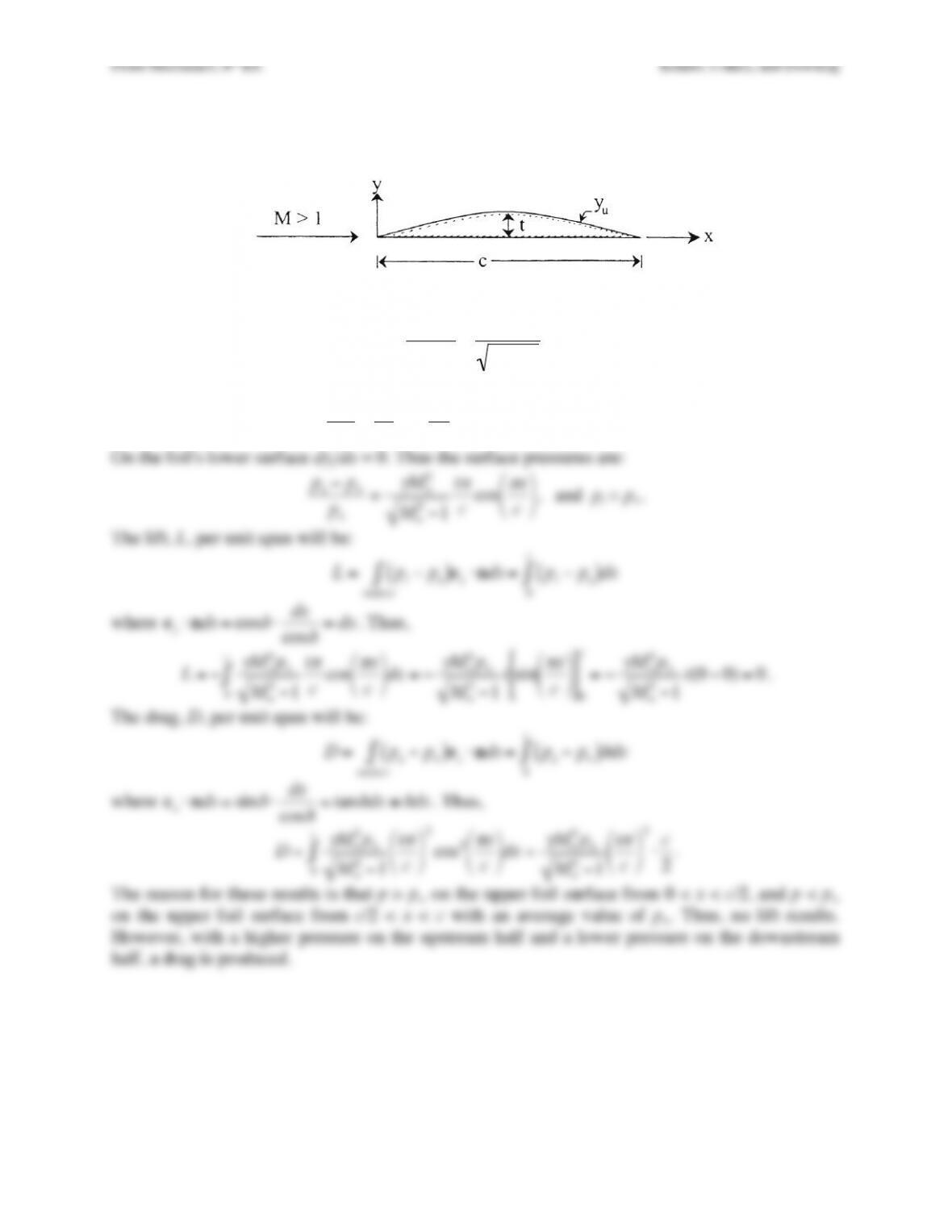
Exercise 15.26. Using thin airfoil theory calculate the lift and drag on the airfoil shape given by
yu = t sin(
π
x/c) for the upper surface and y1 = 0 for the lower surface. Assume a supersonic
stream parallel to the x-axis. The thickness ratio t/c << 1.
Solution 15.26. From supersonic thin airfoil theory
p−p∞
p∞
=
γ
M∞
2
δ
M∞
2−1
,
where
δ
is the slope of the streamline on the surface of the foil. On the foil’s upper surface:
dyu
dx =t
π
c
cos
π
x
c
#
$
% &
‘
( =tan
δ
≅
δ
for
δ
<< 1.
On the foil’s lower surface dyl/dx = 0. Thus the surface pressures are:
Fluid Mechanics, 6th Ed. Kundu, Cohen, and Dowling
Exercise 15.27. Consider a thin airfoil with chord length l at a small angle of attack in a
horizontal supersonic flow at speed M∞. The foil’s upper and lower surface contours, yu(x) and
yl(x), respectively, are defined by:
yu(x) = t(x)/2 + yc(x) –
α
x , and yl(x) = –t(x)/2 + yc(x) –
α
x ,
where: t(x) = the foil’s thickness distribution,
α
= the foil’s angle of attack, and yc(x) = the foil’s
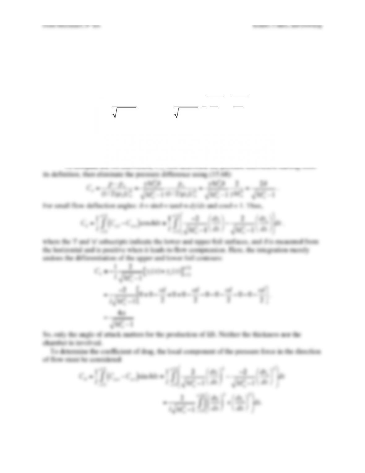
camber line. Use these definitions to show that the foil’s coefficients of lift and drag are:
CL=4
α
M∞
2−1
, and
CD=4
M∞
2−1
1
4
dt
dx
#
$
%&
‘
(
2
+dyc
dx
#
$
%&
‘
(
2
+
α
2
)
*
+
+
,
–
.
.
.
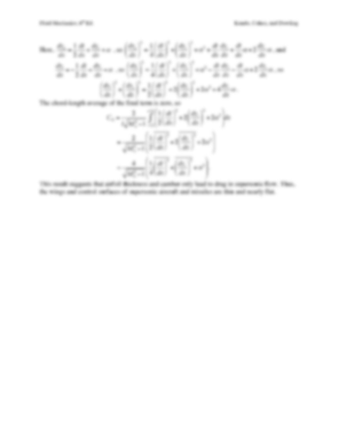
Solution 15.27. Use x–y coordinates and assume the foil extends x = –l/2 to x = +l/2. For
geometrical consistency, the upper and lower foil-surface contours must match at the foil’s
leading and trailing edges: yu(–l/2) = yl(–l/2), and yu(+l/2) = yl(+l/2), so t(–l/2) = t(+l/2) = 0.
And, by definition, yc(–l/2) = yc(+l/2) = 0.
To compute the lift coefficient, CL, first determine the pressure coefficient starting from
Fluid Mechanics, 6th Ed. Kundu, Cohen, and Dowling