Fluid Mechanics, 6th Ed. Kundu, Cohen, and Dowling
Exercise 15.1. Use (15.4), (15.5), and (15.6) to derive (15.7) when the body force is spatially
uniform and the effects of viscosity are negligible.
Solution 15.1. The goal is develop an equation with an inhomogeneous-medium convected-wave
operator acting on p on the left side with source terms involving q, fi, and ∂ui/∂xj on the right.
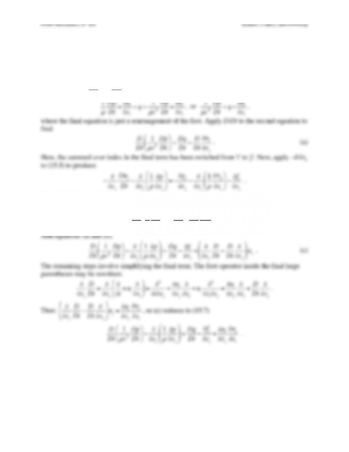
First, use (15.6),
Dp
Dt =c2D
ρ
Dt
, to eliminate D
ρ
/Dt from (15.4):
1
ρ
D
ρ
Dt +∂ui
∂xi
=q=1
ρ
c2
Dp
Dt +∂ui
∂xi
, or
1
ρ
c2
Dp
Dt =q−∂ui
∂xi
,
where the final equation is just a rearrangement of the first. Apply D/Dt to the second equation to
find:
D
Dt
1
ρ
c2
Dp
Dt
!
“
#$
%
&=Dq
Dt −D
Dt
∂uj
∂xj
. (a)
Here, the summed-over index in the final term has been switched from ‘i‘ to ‘j‘. Next, apply –∂/∂xj
to (15.5) to produce:
−∂
∂xj
Duj
Dt −∂
∂xj
1
ρ
∂p
∂xj
#
$
%
%
&
‘
(
(=−∂gj
∂xj
−∂
∂xj
1
ρ
∂
τ
ij
∂xi
#
$
%&
‘
(−∂fi
∂xj
.
Note that ∂gj/∂xj = 0 because the body force is spatially uniform, drop the viscous stress term,
and move the remaining term that explicitly involves uj to the right side:
−∂
∂xj
1
ρ
∂p
∂xj
#
$
%
%
&
‘
(
(=−∂fi
∂xj
+∂
∂xj
Duj
Dt
. (b)
Add equations (a) and (b):
Fluid Mechanics, 6th Ed. Kundu, Cohen, and Dowling
Exercise 15.2. Derive (15.12) through the following substitution and linearization steps. Set q
and fi to zero in (15.7) and insert the decompositions (15.9). Treat Ui, p0,
ρ
0 and T0 as time-
invariant and spatially uniform, and drop quadratic and higher order terms involving the
fluctuations
!
ui
, p´,
ρ
´, and T´.
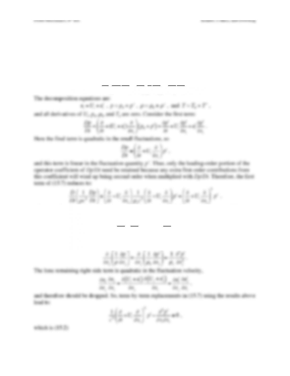
Solution 15.2. Start with (15.7) and set q and fi to zero. This leaves:
D
Dt
1
ρ
c2
Dp
Dt
!
“
#$
%
&−∂
∂xj
1
ρ
∂p
∂xj
!
“
#
#
$
%
&
&=∂ui
∂xj
∂uj
∂xi
.
The decomposition equations are:
where c is the speed of sound at pressure p0 and temperature T0. The second term simplifies in a
similar manner:
∂p
∂xj
=∂
∂xj
p0+“
p
( )
=∂“
p
∂xj
.
Again this term is linear in the fluctuation quantity p´, so its coefficient cannot contain any first-
order contributions from fluctuation quantities
∂
∂xj
1
ρ
∂p
∂xj
“
#
$
$
%
&
‘
‘≅∂
∂xj
1
ρ
0
∂)
p
∂xj
“
#
$
$
%
&
‘
‘=1
ρ
o
∂2)
p
∂xj
2
.
The lone remaining right-side term is quadratic in the fluctuation velocity,
∂ui
∂xj
∂uj
∂xi
=∂Ui+“
ui
( )
∂xj
∂Uj+“
uj
( )
∂xi
=∂“
ui
∂xj
∂“
uj
∂xi
,
and therefore should be dropped. So, term-by-term replacements in (15.7) using the results above
lead to:
1
c2
∂
∂
t+Ui
∂
∂
xi
!
“
#$
%
&
2
‘
p−
∂
2‘
p
∂
xi
∂
xi
≅0
,
which is (15.2)
Fluid Mechanics, 6th Ed. Kundu, Cohen, and Dowling
Exercise 15.3. The field equation for acoustic pressure fluctuations in an ideal compressible
fluid is (15.13). Consider one-dimensional solutions where p = p(x,t) and x = x1.
a) Drop the x2 and x3 dependence in (15.13), and change the independent variables x and t to
ξ
=x−ct
and
ζ
=x+ct
to simplify (15.13) to
∂
2#
p
∂ξ∂ζ
=0
.
b) Use the simplified equation in part a) to find the general solution to the original field equation:
“
p (x,t)=f(x−ct)+g(x+ct)
where f and g are undetermined functions.
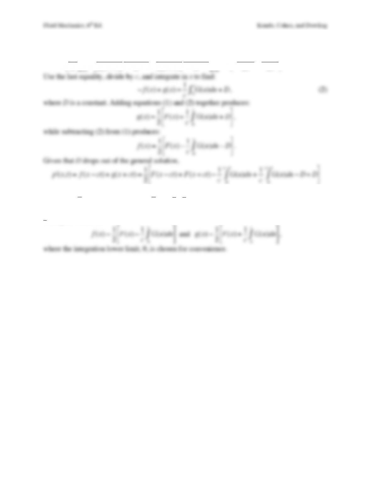
c) When the initial conditions are: p´ = F(x) and ∂p´/∂t = G(x) at t = 0, show that:
f(x)=1
2F(x)−1
cG(x )dx
0
x
∫
$
%
&
‘
(
)
, and
g(x)=1
2F(x)+1
cG(x )dx
0
x
∫
#
$
%
&
‘
(
,
where x is just an integration variable.
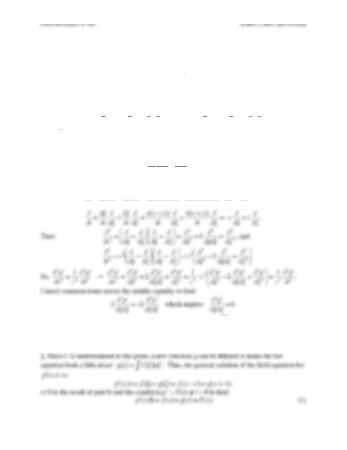
Solution 15.3. a) The starting point is (15.13) simplified for no x2 and x3 dependence. This is the
classical one-dimensional acoustic wave equation,
1
c2
∂
2#
p
∂
t2−
∂
2#
p
∂
x2=0
.
Use
ξ
=x−ct
and
ζ
=x+ct
, and convert the partial derivatives with respect to x and t into
partial derivatives with respect to
ξ
and
ζ
.
∂
∂
x=
∂ξ
∂
x
∂
∂ξ
+
∂ζ
∂
x
∂
∂ζ
=
∂
(x−ct)
∂
x
∂
∂ξ
+
∂
(x+ct)
∂
x
∂
∂ζ
=
∂
∂ξ
+
∂
∂ζ
, and
∂
∂
t=
∂ξ
∂
t
∂
∂ξ
+
∂ζ
∂
t
∂
∂ζ
=
∂
(x−ct)
∂
t
∂
∂ξ
+
∂
(x+ct)
∂
t
∂
∂ζ
=−c
∂
∂ξ
+c
∂
∂ζ
.
Thus:
∂
2
∂
x2=
∂
∂ξ
+
∂
∂ζ
%
&
‘
(
)
*
∂
∂ξ
+
∂
∂ζ
%
&
‘
(
)
* =
∂
2
∂ξ
2+2
∂
2
∂ξ∂ζ
+
∂
2
∂ζ
2
, and
∂
2
∂
t2=c2
∂
∂ξ
−
∂
∂ζ
&
‘
(
)
*
+
∂
∂ξ
−
∂
∂ζ
&
‘
(
)
*
+ =c2
∂
2
∂ξ
2−2
∂
2
∂ξ∂ζ
+
∂
2
∂ζ
2
&
‘
(
)
*
+
So,
∂
2#
p
∂
x2=1
c2
∂
2#
p
∂
t2
→
∂
2$
p
∂
x2=
∂
2$
p
∂ξ
2+2
∂
2$
p
∂ξ∂ζ
+
∂
2$
p
∂ζ
2=1
c2⋅c2
∂
2$
p
∂ξ
2−2
∂
2$
p
∂ξ∂ζ
+
∂
2$
p
∂ζ
2
)
*
+
,
–
. =1
c2
∂
2$
p
∂
t2
.
Cancel common terms across the middle equality to find:
2
∂
2#
p
∂ξ∂ζ
=−2
∂
2#
p
∂ξ∂ζ
which implies
∂
2#
p
∂ξ∂ζ
=0
.
b) Use the result of part a) and integrate with respect to
ξ
to find:
∂
#
p
∂ζ
=C
ζ
( )
where C(
ζ
) is a
function of integration that cannot depend on
ξ
. Now integrate this result with respect to
ζ
to
find:
“
p =C
ζ
( )
∫d
ζ
+f(
ξ
)
where f(
ξ
) is a second function of integration that cannot depend on
ζ
. Since C is undetermined at this point, a new function g can be defined to make the last
Fluid Mechanics, 6th Ed. Kundu, Cohen, and Dowling
Differentiate the result of part b) with respect to time and use the ∂p´/∂t = G(x) at t = 0 to find:
∂
#
p
∂
t
$
%
&
‘
(
)
t=0
=df
d(x−ct)
∂
(x−ct)
∂
t+df
d(x+ct)
∂
(x+ct)
∂
t
$
%
&
‘
(
)
t=0
=c−df (x)
dx +dg(x)
dx
+
,
– .
/
0 =G(x)
.
Use the last equality, divide by c, and integrate in x to find:
Fluid Mechanics, 6th Ed. Kundu, Cohen, and Dowling
Exercise 15.4. Starting from (15.15) use (15.14) to prove (15.16)
Solution 15.4. Equation (15.15) is
“
p (x,t)=f(x−ct)+g(x+ct)
,
and (15.14) is the linearized integrated Euler equation without the body force:
“
u
1(x,t)=−1
ρ
o
∂
“
p
∂
xdt
∫
.
Substitute (15.15) into (15.14), define the variables
ξ
=x−ct
and
ζ
=x+ct
, and note that
Fluid Mechanics, 6th Ed. Kundu, Cohen, and Dowling
Exercise 15.5. Consider two approaches to determining the upper Mach number limit for
incompressible flow.
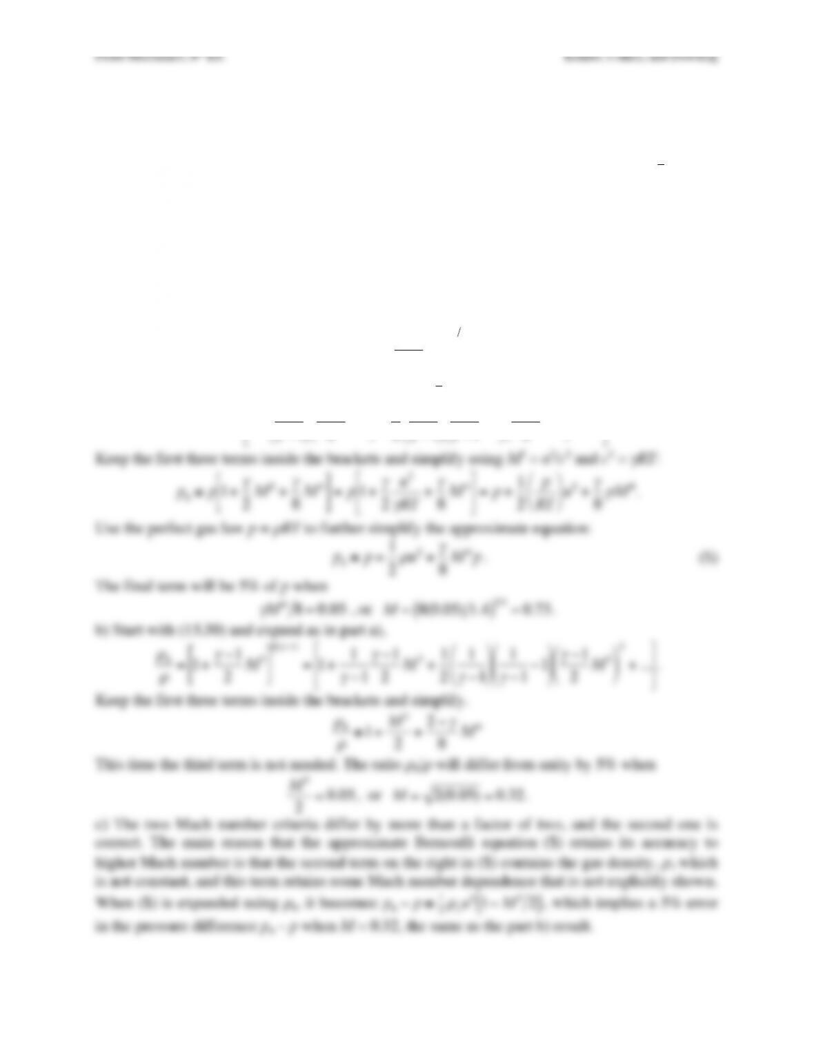
a) First consider pressure errors in the simplest-possible steady flow Bernoulli equation. Expand
(15.29) for small Mach number to determine the next term in the expansion:
p0=p+1
2
ρ
u2+…
and determine the Mach number at which this next term is 5% of p when
γ
= 1.4.
b) Second consider changes to the density. Expand (15.30) for small Mach number and
determine the Mach number at which the density ratio
ρ
0/
ρ
differs from unity by 5% when
γ
=
1.4.
c) Which criterion is correct? Explain why the criteria for incompressibility determined in a) and
b) differ, and reconcile them if you can.
Solution 15.5. a) Start with (15.29),
p0=p1+
γ
−1
2M2
$
%
&
‘
(
)
γ
(
γ
−1)
,
and expand using the Taylor series
(1+
ε
)
β
=1+
βε
+1
2
β
(
β
−1)
ε
2+…
for
ε
<< 1:
p0=p1+
γ
γ
−1
$
%
&
‘
(
)
γ
−1
2M2
$
%
& ‘
(
) +1
2
γ
γ
−1
$
%
&
‘
(
)
γ
γ
−1−1
$
%
&
‘
(
)
γ
−1
2M2
$
%
& ‘
(
)
2
+…
*
+
,
–
.
/
.
Keep the first three terms inside the brackets and simplify using M2 = u2/c2 and c2 =
γ
RT:
Fluid Mechanics, 6th Ed. Kundu, Cohen, and Dowling
Exercise 15.6. The critical area A∗ of a duct flow was defined in §4. Show that the relation
between A∗ and the actual area A at a section, where the Mach number equals M, is that given by
(15.31). This relation was not proved in the text. [Hint: Write
A
A*=
ρ
*c*
ρ
u=
ρ
*
ρ
0
ρ
0
ρ
c*
c
c
u=
ρ
*
ρ
0
ρ
0
ρ
T*
T0
T0
T
1
M
.
Then use the other relations given in Section 15.4.]
Solution 15.6. Start with the hint and continue the equality, noting that M* = 1 and using (15.28)
and (15.30)
A
A*=
ρ
*
ρ
0
ρ
0
ρ
T*
T0
T0
T
1
M
=1+
γ
−1
2
M*2
%
&
‘
(
)
*
−1
γ
−1
1+
γ
−1
2
M2
%
&
‘
(
)
*
1
γ
−1
1+
γ
−1
2
M*2
%
&
‘
(
)
*
−1
2
1+
γ
−1
2
M2
%
&
‘
(
)
*
1
21
M
=1+
γ
−1
2
%
&
‘
(
)
*
−1
γ
−1
1+
γ
−1
2
M2
%
&
‘
(
)
*
1
γ
−1
1+
γ
−1
2
%
&
‘
(
)
*
−1
2
1+
γ
−1
2
M2
%
&
‘
(
)
*
1
21
M
=
γ
+1
2
%
&
‘
(
)
*
−1
γ
−1
1+
γ
−1
2
M2
%
&
‘
(
)
*
1
γ
−1
γ
+1
2
%
&
‘
(
)
*
−1
2
1+
γ
−1
2
M2
%
&
‘
(
)
*
1
21
M
=
γ
+1
2
%
&
‘
(
)
*
−1
γ
−1+1
2
+
,
–
.
/
0
1+
γ
−1
2
M2
%
&
‘
(
)
*
+1
γ
−1+1
2
+
,
–
.
/
0 1
M=2
γ
+1
1+
γ
−1
2
M2
+
,
– .
/
0
%
&
‘
(
)
*
+1
2
γ
+1
γ
−1
+
,
–
.
/
0
.
Fluid Mechanics, 6th Ed. Kundu, Cohen, and Dowling
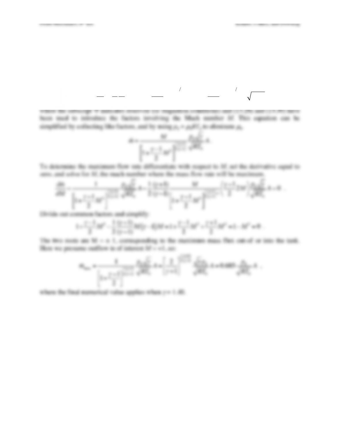
Exercise 15.7. A perfect gas is stored in a large tank at the conditions specified by p0, T0.
Calculate the maximum mass flow rate that can exhaust through a duct of cross-sectional area A.
Assume that A is small enough that during the time of interest p0 and T0 do not change
significantly and that the flow is isentropic.
Solution 15.7. The mass flux through the tube will be:
!
m=
ρ
UA =
ρ
ρ
0
ρ
0
U
c
c
c0
c0A=1+
γ
−1
2
M2
“
#
$%
&
‘
−1 (
γ
−1)
M1+
γ
−1
2
M2
“
#
$%
&
‘
−1 2
ρ
0
γ
RT0A
,
where the subscript ‘0’ indicates reservoir (or stagnation conditions) and (15.28) and (15.30) have
Fluid Mechanics, 6th Ed. Kundu, Cohen, and Dowling
Exercise 15.8. The entropy change across a normal shock is given by (15.43). Show that this
reduces to expressions (15.44) for weak shocks. [Hint: Let
M1
2−1
<< 1. Write the terms within
the two sets of brackets in equation (15.43) in the form [1 +
ε
1] [1 +
ε
2]
γ
, where
ε
1 and
ε
2 are
small quantities. Then use the series expansion ln(1 +
ε
) =
ε
–
ε
2/2 +
ε
3/3 + … . This gives
equation (15.44) times a function of M1 which can be evaluated at M1 = 1.]
Solution 15.8. From (15.43)
S2−S1
cv
=ln 1+2
γ
γ
+1
M1
2−1
( )
“
#
$%
&
‘(
γ
−1)M1
2+2
(
γ
+1)M1
2
“
#
$%
&
‘
γ
(
)
*
+
*
,
–
*
.
*
.
The term in the first set of [,]-brackets is already in an easily managed form:
1+2
γ
γ
+1
M1
2−1
( )
≡1+
ε
1
.
The term in the second set of [,]-brackets can be rearranged as follows:
(
γ
−1)M1
2+2
(
γ
+1)M1
2=(
γ
+1)M1
2−2M1
2+2
(
γ
+1)M1
2=1−2(M1
2−1)
(
γ
+1)M1
2≡1−
ε
2
.
Together these two results produce:
S2−S1
cv
=ln 1+
ε
1
[ ]
1+
ε
2
[ ]
γ
{ }
=ln 1+
ε
1
( )
+
γ
ln 1−
ε
2
( )
.
Now expand the natural logarithm functions:
S2−S1
cv
=
ε
1−
ε
1
2
2+
ε
1
3
3+… +
γ
−
ε
2−
ε
2
2
2−
ε
2
3
3+…
“
#
$%
&
‘
≅(
ε
1−
γε
2)−1
2
ε
1
2+
γε
2
2
( )
+1
3
ε
1
3−
γε
2
3
( )
.
Evaluate the terms.
ε
1−
γε
2=2
γ
γ
+1
M1
2−1
( )
−
γ
2(M1
2−1)
(
γ
+1)M1
2=2
γ
(M1
2−1)
γ
+11−1
M1
2
%
&
‘
(
)
* =2
γ
(M1
2−1)2
(
γ
+1)M1
2
1
2
ε
1
2+
γε
2
2
( )
=1
2
4
γ
2
(
γ
+1)2M1
2−1
( )
2+
γ
4(M1
2−1)2
(
γ
+1)2M1
4
%
&
‘
(
)
* =2
γ
(
γ
+1)2M1
2−1
( )
2
γ
+1
M1
4
+
,
–
.
/
0
1
3
ε
1
3−
γε
2
3
( )
=1
3
8
γ
3
(
γ
+1)3M1
2−1
( )
3−
γ
8(M1
2−1)3
(
γ
+1)3M1
6
%
&
‘
(
)
* =8
γ
3(
γ
+1)3M1
2−1
( )
3
γ
2−1
M1
6
+
,
–
.
/
0
Reconstruct the entropy difference and simplify.
S2−S1
cv
≅2
γ
(M1
2−1)2
(
γ
+1)M1
2−2
γ
(M1
2−1)2
(
γ
+1)2
γ
+1
M1
4
#
$
%&
‘
(+8
γ
(M1
2−1)3
3(
γ
+1)3
γ
2−1
M1
6
#
$
%&
‘
(
=2
γ
(M1
2−1)2
(
γ
+1)
1
M1
2−
γ
γ
+1−1
(
γ
+1)M1
4+4(M1
2−1)
3(
γ
+1)2
γ
2−4(M1
2−1)
3(
γ
+1)2M1
6
#
$
%&
‘
(
=2
γ
(M1
2−1)2
(
γ
+1)
3(
γ
+1)2M1
2−3
γ
(
γ
+1)M1
4−3(
γ
+1) +4(M1
2−1)
γ
2M1
4−4(M1
2−1)M1
−2
3(
γ
+1)2M1
4
#
$
%&
‘
(
Fluid Mechanics, 6th Ed. Kundu, Cohen, and Dowling
S2−S1
cv
≅2
γ
(M1
2−1)2
(
γ
+1)
3(
γ
+1) (−
γ
M1
2+1)(M1
2−1)
#
$%
&+4(M1
2−1)
γ
2M1
4−4(M1
2−1)M1
−2
3(
γ
+1)2M1
4
#
$
‘
‘
%
&
(
(
=2
γ
(M1
2−1)3
(
γ
+1)
3(
γ
+1)(−
γ
M1
2+1) +4
γ
2M1
4−4M1
−2
3(
γ
+1)2M1
4
#
$
‘%
&
(
Given that the first term is cubic in the small quantity, the contents of the final [,]-brackets can be
evaluated at M1 = 1. This produces:
S2−S1
cv
≅2
γ
(M1
2−1)3
(
γ
+1)
3(
γ
+1)(−
γ
+1) +4
γ
2−4
3(
γ
+1)2
#
$
%&
‘
(=2
γ
(M1
2−1)3
(
γ
+1)
3(−
γ
+1) +4
γ
−4
3(
γ
+1)
#
$
%&
‘
(
=2
γ
(M1
2−1)3
(
γ
+1)
γ
−1
3(
γ
+1)
#
$
%&
‘
(=2
γ
(
γ
−1)
3(
γ
+1)2(M1
2−1)3,
which is (15.44a).
Fluid Mechanics, 6th Ed. Kundu, Cohen, and Dowling
Exercise 15.9. Show that the maximum velocity generated from a reservoir in which the
stagnation temperature equals T0 is
umax =2cpTo
. What are the corresponding values of T and
M?
Solution 15.9. If the flow starts from zero velocity within a reservoir is T0, then the energy
equation is:
Fluid Mechanics, 6th Ed. Kundu, Cohen, and Dowling
Exercise 15.10. In an adiabatic flow of air through a duct, the conditions at two points are u1 =
250 m/s, T1 = 300 K, p1 = 200 kPa, u2 = 300 m/s, p2 = 150 kPa. Show that the loss of stagnation
pressure is nearly 34.2 kPa. What is the entropy increase?
Solution 15.10. First, compute the speed of sound at the upstream location:
c1=
γ
RT
1=(1.4)(287)(300) =347.2ms−1
.
Therefore, the mach number is: M1 = u1/c1 = 250/347.2 = 0.72. From table 15.1,
Fluid Mechanics, 6th Ed. Kundu, Cohen, and Dowling
Exercise 15.11. A shock wave generated by an explosion propagates through a still atmosphere.
If the pressure downstream of the shock wave is 700 kPa, estimate the shock speed and the flow
velocity downstream of the shock.
Solution 15.11. The analysis can be done in a shock-fixed frame of reference, and p1 = 101.3 kPa
and T1 = 295K, are taken as the nominal atmospheric conditions. The shock’s pressure ratio is:
p2
p1
=700kPa
101.3kPa =6.91
.
Locating the closest value in Table 15.2 produces:
Fluid Mechanics, 6th Ed. Kundu, Cohen, and Dowling
Exercise 15.12. Prove the following formulae for the jump the conditions across a stationary
normal shock wave:
p2−p1
p1
=2
γ
γ
+1
M1
2−1
( )
,
u2−u1
c1
=−2
γ
+1
M1−1
M1
“
#
$%
&
‘
, and
υ
2−
υ
1
υ
1
=−2
γ
+1
1−1
M1
2
“
#
$%
&
‘
,
where
υ
= 1/
ρ
, and the subscripts ‘1’ and ‘2’ imply upstream and downstream conditions,
respectively.
Solution 15.12. The pressure ratio condition (15.39) is:
p2
p1
=1+2
γ
γ
+1M1
2−1
“
#$
%
.
Subtract ‘1’ from both sides, and rearrange on the left to find:
Fluid Mechanics, 6th Ed. Kundu, Cohen, and Dowling
Exercise 15.13. Using (15.1i), and (15.43), determine formulae for p02/p01 and
ρ
02/
ρ
01 for a
normal shock wave in terms of M1 and
γ
. Is there anything notable about the results?
Solution 15.13. Equation (15.1i) applied to stagnation conditions implies:
s2−s1
cp
=ln T02
T01
“
#
$%
&
‘−R
cp
ln p02
p01
“
#
$%
&
‘
Flow through the shock wave is adiabatic so T02 = T01, and
s2−s1
cp
=−R
cp
ln p02
p01
“
#
$%
&
‘=cv
cp
ln 1+2
γ
γ
+1M1
2−1
( )
(
)
*+
,
–(
γ
−1)M1
2+2
(
γ
+1)M1
2
“
#
$%
&
‘
γ
.
/
0
1
0
2
3
0
4
0
.
A little algebraic rearrangement using (15.1d) and (15.1g) leads to:
p02
p01
=1+2
γ
γ
+1M1
2−1
( )
“
#
$%
&
‘
−1
γ
−1(
γ
+1)M1
2
(
γ
−1)M1
2+2
(
)
*+
,
–
γ
γ
−1
.
The formula for the stagnation density can be found similarly. Equation (15.1i) applied to
stagnation conditions implies:
s2−s1
cv
=ln T02
T01
“
#
$%
&
‘−R
cv
ln
ρ
02
ρ
01
“
#
$%
&
‘
Flow through the shock wave is adiabatic so T02 = T01, and
s2−s1
cv
=−R
cv
ln
ρ
02
ρ
01
“
#
$%
&
‘=ln 1+2
γ
γ
+1
M1
2−1
( )
(
)
*+
,
–(
γ
−1)M1
2+2
(
γ
+1)M1
2
“
#
$%
&
‘
γ
.
/
0
1
0
2
3
0
4
0
.
A little algebraic rearrangement using (15.1d) and (15.1g) leads to:
ρ
02
ρ
01
=1+2
γ
γ
+1
M1
2−1
( )
“
#
$%
&
‘
−1
γ
−1(
γ
+1)M1
2
(
γ
−1)M1
2+2
(
)
*+
,
–
γ
γ
−1
.
Yes, the results are ‘notable’ because they are exactly the same.
Fluid Mechanics, 6th Ed. Kundu, Cohen, and Dowling
Exercise 15.14. Using dimensional analysis, G. I. Taylor deduced that the radius r(t) of the blast
wave from a large explosion would be proportional to (E/
ρ
1)1/5t2/5 where E is the explosive
energy,
ρ
1 is the quiescent air density ahead of the blast wave, and t is the time since the blast
(see Example 1.10). The goal of this problem is to (approximately) determine the constant of
proportionality assuming perfect-gas thermodynamics.
a) For the strong shock limit where
M1
2>>1
, show:
<Begin Equation>
ρ
2
ρ
1
≅
γ
+1
γ
−1
,
T2
T
1
≅
γ
−1
γ
+1
p2
p1
, and
u1=M1c1≅
γ
+1
2
p2
ρ
1
.
</End Equation>
b) For a perfect gas with internal energy per unit mass e, the internal energy per unit volume is
ρ
e. For a hemispherical blast wave, the volume inside the blast wave will be
2
3
π
r3
. Thus, set
ρ
2e2=E2
3
π
r3
, determine p2, set u1 = dr/dt, and integrate the resulting first-order differential
equation to show that r(t) = K(E/
ρ
1)1/5t2/5 when r(0) = 0 and K is a constant that depends on
γ
.
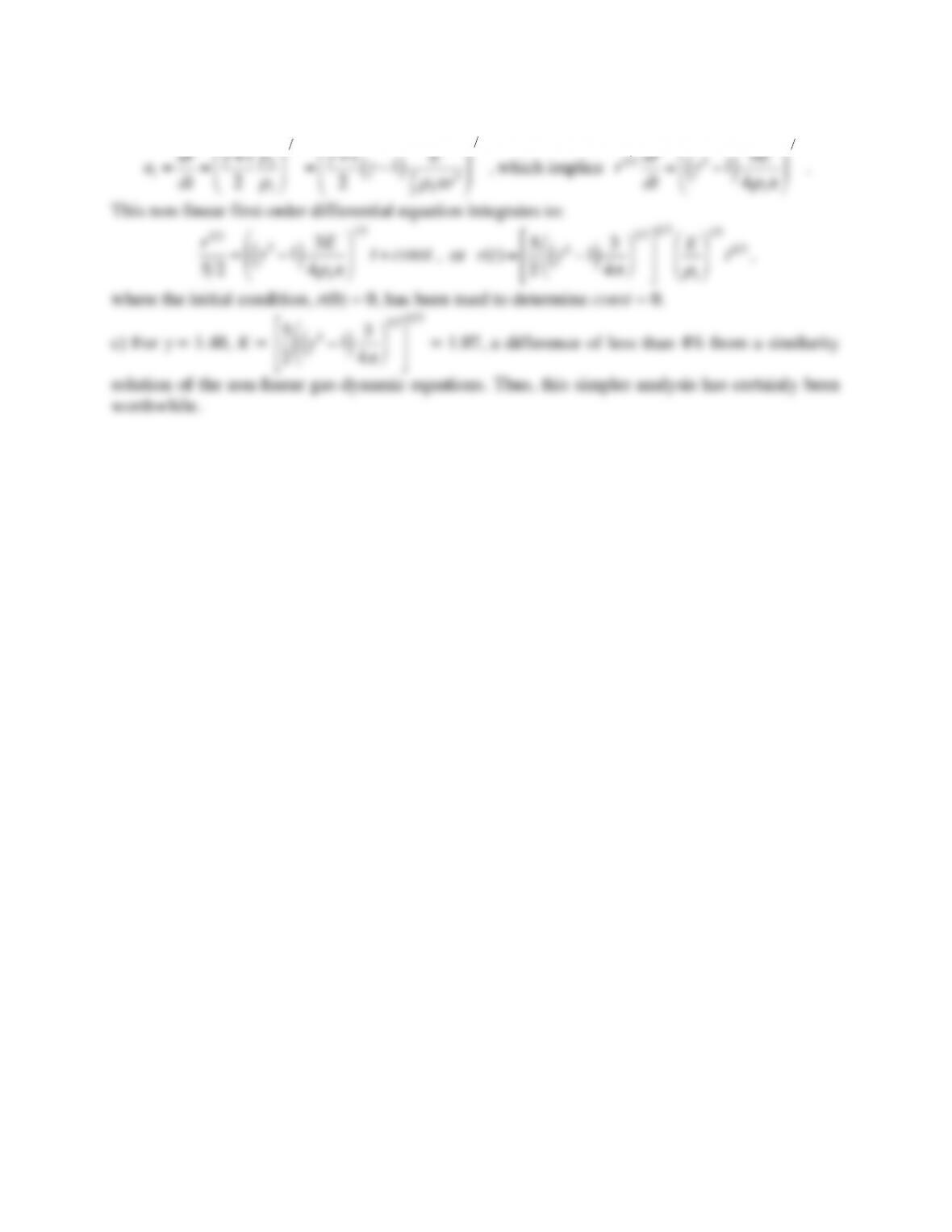
c) Evaluate K for
γ
= 1.4. A full similarity solution of the non-linear gas-dynamic equations in
spherical coordinates produces K = 1.033 for
γ
= 1.4 (see Thompson 1972, p. 501). What is the
percentage error in this exercise’s approximate analysis?
Solution 15.14. Start from the normal shock jump conditions (15.39) – (15.42):
p2
p1
=1+2
γ
γ
+1M1
2−1
( )
,
M2
2=1+
γ
−1
2
M1
2
$
%
& ‘
(
)
γ
M1
2−
γ
−1
2
$
%
& ‘
(
)
,
ρ
2
ρ
1
=(
γ
+1)M1
2
(
γ
−1)M1
2+2
, and
T2
T
1
=1+2(
γ
−1)
(
γ
+1)2
γ
M1
2+1
M1
2
$
%
&
‘
(
) M1
2−1
( )
.
Simplify these four equations for
M1
2>> 1
,
which is another result in the correct form. To reach the final part a) result, invert the strong-
shock pressure relationship to find and expression for M1:
M1≅
γ
+1
2
γ
p2
p1
$
&
‘
)
1 2
, so that
u1=M1c1≅
γ
+1
p2
“
$%
‘
1 2
γ
RT
1=
γ
+1
p2
“
$%
‘
1 2
γ
p1
=
γ
+1
p2
“
$%
‘
1 2
,
Fluid Mechanics, 6th Ed. Kundu, Cohen, and Dowling
Put this into the final result of part a) and set u1 = dr/dt to find:
u1=dr
γ
+1
p2
!
#$
&
1 2
=
γ
+1
γ
−1
( )
E
2
!
#
#
$
&
&
1 2
, which implies
r3 2 dr
γ
2−1
( )
3E
“
$%
‘
1 2
.