Fluid Mechanics, 6th Ed. Kundu, Cohen, and Dowling
Exercise 12.37. The cross-section averaged flow speed Uav in a round pipe of radius a may be
written:
Uav ≡volume flux
area =1
π
a2U(y)2
π
r dr
0
a
∫=2
a2U(y)(a−y)dy
0
a
∫
,
where r is the radial distance from the pipe’s centerline, and y = a – r is the distance inward from
the pipe’s wall. Turbulent pipe flow has very little wake, and the viscous sublayer is very thin at
high Reynolds number; therefore assume the log-law profile,
U(y)=u*
κ
( )
ln yu*
ν
( )
+B
, holds
throughout the pipe to find
Uav ≅u*1
κ
( )
ln au*
ν
( )
+B−3 2
κ
#
$%
&
.
Now use the definitions:
Cf=
τ
w
1
2
ρ
Uav
2
,
Red=2Uav a
ν
,
f=4Cf=
the Darcy friction factor,
κ
= 0.41, B = 5.0, and switch to base-10 logarithms to reach (12.105).
Solution 12.37. Start with given relationships and integrate:
Uav =2
a2U(y)(a−y)dy
0
a
∫≅2
a2
u*
κ
ln yu*
ν
‘
(
) *
+
, +u*B
–
.
/
0
1
2
(a−y)dy
0
a
∫
=2
ν
a2
κ
u*a
ν
ln yu*
ν
‘
(
) *
+
, −u*y
ν
ln yu*
ν
‘
(
) *
+
,
–
.
/
0
1
2
dy
0
a
∫+2u*B
a2a−y
[ ]
dy
0
a
∫
=2
ν
2
a2
κ
u*
au*
ν
ln
β
( )
−
β
ln
β
( )
–
.
/
0
1
2
d
β
0
au*
ν
∫+2u*B
a2ay −y2
2
–
.
/
0
1
2
0
a
=2
ν
2
a2
κ
u*
au*
νβ
ln
β
−
β
( )
−
β
2
2ln
β
( )
+
β
2
4
–
.
/
0
1
2
0
au*
ν
+2u*B
a2a2−a2
2
–
.
/
0
1
2
=2
ν
2
a2
κ
u*
au*
ν
au*
ν
ln au*
ν
−au*
ν
‘
(
) *
+
, −1
2
au*
ν
‘
(
) *
+
,
2
ln au*
ν
‘
(
) *
+
, +1
4
au*
ν
‘
(
) *
+
,
2
–
.
/
0
1
2
+u*B
=2
ν
2
a2
κ
u*
1
2
au*
ν
‘
(
) *
+
,
2
ln au*
ν
‘
(
) *
+
, −3
4
au*
ν
‘
(
) *
+
,
2
–
.
/
0
1
2
+u*B=u*
1
κ
ln au*
ν
‘
(
) *
+
, −3
2
κ
+B
‘
(
) *
+
,
.
The second part of this exercise is primarily algebraic. Start by rewriting the ratio Uav/u* in terms
of
f
, and rewriting the ratio u*a/
ν
in terms of Red and
f
:
Uav
u*
=Uav
τ
w
ρ
=Uav
1
2CfUav
2=1
1
8f
=8
f1 2
, and
au*
ν
=
2aUav
1
8f
2
ν
=1
32 f 1 2 Red
.
Put these into the result of part a) and recall that ln(…) = ln(10)log10(…).
Fluid Mechanics, 6th Ed. Kundu, Cohen, and Dowling
Exercise 12.38. The cross-section averaged flow speed Uav in a wide channel of full height b
may be written:
Uav ≡2
bU(y)dy
0
b2
∫
,
where y is the vertical distance from the channel’s lower wall. Turbulent channel flow has very
little wake, and the viscous sublayer is very thin at high Reynolds number; therefore assume the
log-law profile,
U(y)=u*
κ
( )
ln yu*
ν
( )
+B
, holds throughout the channel to find
Uav ≅u*1
κ
( )
ln bu*2
ν
( )
+B−1
κ
#
$%
&
.
Now use the definitions:
Cf=
τ
w
1
2
ρ
Uav
2
,
Reb=Uav b
ν
,
f=4Cf=
the Darcy friction factor,
κ
= 0.41, B = 5.0, and switch to base-10 logarithms to reach:
f−1 2 =2.0 log10 Rebf1 2
( )
−0.59
.
Solution 12.38. Start with given relationships and integrate:
Uav =2
bU(y)dy
0
b2
∫≅2
b
u*
κ
ln yu*
ν
#
$
%&
‘
(+u*B
)
*
+,
–
.dy
0
b2
∫
=2
ν
b
κ
u*
ν
ln yu*
ν
#
$
%&
‘
(dy
0
b2
∫+2u*B
bdy
0
b2
∫=2
ν
b
κ
ln
β
( )
d
β
0
bu*2
ν
∫+2u*B
b
b
2
=2
ν
b
κβ
ln
β
−
β
[ ]
0
bu*2
ν
+u*B=2
ν
b
κ
bu*
2
ν
ln bu*
2
ν
#
$
%&
‘
(−bu*
2
ν
#
$
%&
‘
(+u*B
=u*
1
κ
ln bu*
2
ν
#
$
%&
‘
(−1
κ
+B
#
$
%&
‘
(.
The second part of this exercise is primarily algebraic. Start by rewriting the ratio Uav/u* in terms
of
f
, and rewriting the ratio u*b/2
ν
in terms of Reb and
f
:
Uav
u*
=Uav
τ
w
ρ
=Uav
1
2CfUav
2=1
1
8f
=8
f1 2
, and
bu*
2
ν
=bUav
1
8f
2
ν
=1
32 f1 2 Reb
.
Put these into the result of part a) and recall that ln(…) = ln(10)log10(…).
Uav
u*
=1
κ
ln bu*
2
ν
!
“
#$
%
&−1
κ
+B→8
f1 2 =ln(10)
κ
log10
1
32 f1 2 Reb
!
“
#$
%
&−1
κ
+B
.
Rearrange to reach the desired form, and evaluate using the numbers provided above.
1
f1 2 =ln(10)
8
κ
log10 f1 2 Reb
( )
+1
8−1
κ
+B−ln 32
κ
“
#
$%
&
‘=1.986 log10 f1 2 Red
( )
−0.589
.
This is the desired result.
Fluid Mechanics, 6th Ed. Kundu, Cohen, and Dowling
Exercise 12.39. For laminar flow, the hydraulic diameter concept is successful when the ratio
f⋅Uavdh
ν
( )
duct f⋅Uavd
ν
( )
round pipe
is near unity. Show that this ratio is 1.5 when the duct is a
wide channel.
Solution 12.39. For a channel with height b and width w, the hydraulic diameter from (12.103)
is:
dh
( )
channel =4bw
2b+2w=2b
1+b w
, and this simplifies to: (dh)channel ≈ 2b when w >> b.
The friction factor is appears in (12.102):
P
u−P
d=1
ρ
Uav
2⋅L
⋅f
, so:
Fluid Mechanics, 6th Ed. Kundu, Cohen, and Dowling
Exercise 12.40. a) Rewrite the final friction factor equation in Exercise 12.38 in terms of the
channel’s hydraulic diameter instead of its height b.
b) Using the friction factor-Reynolds number ratio given in Exercise 12.39, evaluate (12.107) for
a wide channel.
c) Are the results of parts a) and b) in good agreement?
Solution 12.40. a) For a channel with height b and width w, the hydraulic diameter from
(12.103) is:
dh
( )
channel =4bw
2b+2w=2b
1+b w
, and this simplifies to: (dh)channel ≈ 2b when w >> b.
The final result of Exercise 12.38 is
f−1 2 =2.0 log10 Rebf1 2
( )
−0.59
, which can be rewritten:
Fluid Mechanics, 6th Ed. Kundu, Cohen, and Dowling
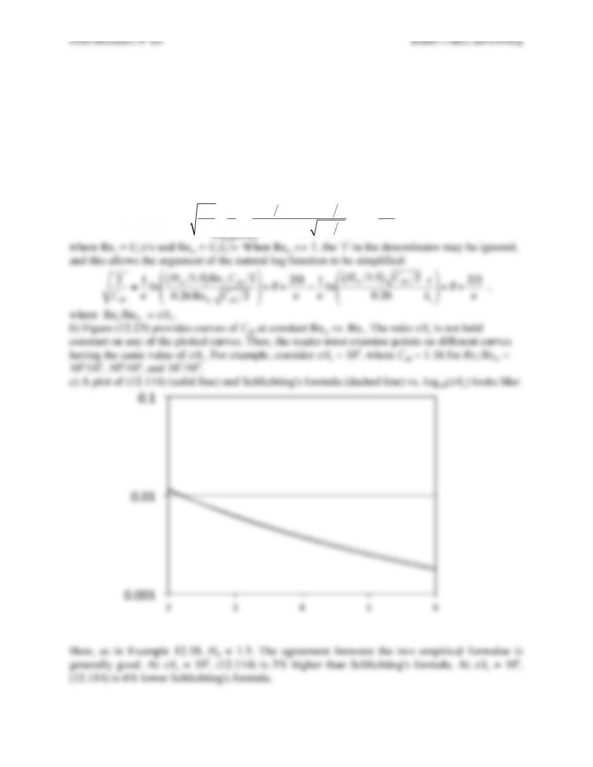
Exercise 12.41. a) Simplify (12.114) when the roughness Reynolds number is large Reks >> 1 to
show that CfR is independent of
ν
in the fully rough regime.
b) Reconcile the finding of part a) with the results in Figure 12.25 which appear to show that CfR
depends on Rex for all values of Reks.
c) For this fully rough regime, compare CfR computed from (12.114) with the empirical formula
provided in Schlichting (1979):
CfR =2.87 +1.58⋅log10 (x/ks)
( )
−2.5
.
Solution 12.41. a) Eq. (12.114) is:
2
CfR
≅1
κ
ln HR3.5
( )
RexCfR 2
1+0.26 Reks CfR 2
“
#
$
$
%
&
‘
‘+B+2Π
κ
,
where Rex = Uex/
ν
and Reks = Ueks/
ν
. When Reks >> 1, the ‘1’ in the denominator may be ignored,
CfR
log10(x/ks)
Fluid Mechanics, 6th Ed. Kundu, Cohen, and Dowling
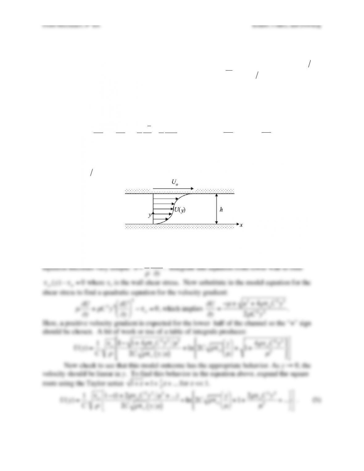
Exercise 12.42. Perhaps the simplest way to model turbulent flow is to develop an eddy
viscosity from dimensional analysis and physical reasoning. Consider turbulent Couette flow
with wall spacing h. Assume that eddies of size l produce velocity fluctuations of size
l
∂
U
∂
y
( )
so that the turbulent shear stress correlation can modeled as:
−uv ∝l2
∂
U
∂
y
( )
2
. Unfortunately, l
cannot be a constant because it must disappear near the walls. Thus, more educated guessing is
needed, so for this problem assume ∂U/∂y will have some symmetry about the channel centerline
(as shown) and try:
l=Cy
for 0 ≤ y ≤ h/2 where C is a positive dimensionless constant and y is
the vertical distance measured from the lower wall. With this turbulence model, the RANS
equation for 0 ≤ y ≤ h/2 becomes:
U
∂
U
∂
x+V
∂
U
∂
y=−1
ρ
dp
dx +1
ρ
∂τ
xy
∂
y
where
τ
xy =
µ∂
U
∂
y+
ρ
C2y2
∂
U
∂
y
%
&
‘
(
)
*
2
Determine an analytic form for U(y) after making appropriate simplifications of the RANS
equation for fully developed flow assuming the pressure gradient is zero. Check to see that your
final answer recovers the appropriate forms as y → 0 and C → 0. Use the fact that
U(y=h/2) =Uo2
in your work if necessary.
Solution 12.42. In Couette flow V will be zero because the fluid is confined and ∂/∂x = 0 because
the flow is homogeneous in this direction. Thus, with zero pressure gradient, the RANS BL
equation becomes very simple:
0=1
ρ
∂τ
xy
∂
y
. Integrate this equation from lower wall to find:
Fluid Mechanics, 6th Ed. Kundu, Cohen, and Dowling
Fluid Mechanics, 6th Ed. Kundu, Cohen, and Dowling
Exercise 12.43. Incompressible, constant-density-and-viscosity, fully-developed, pressure-
gradient-driven, turbulent channel flow is often used to test turbulence models for wall-bounded
flows. Thus, for this flow, investigate the following simplified mixing-length model for the
Reynolds shear stress:
−#
u #
v =
β
y
τ
w
ρ ∂
U
∂
y
( )
for 0 ≤ y ≤ h/2 where y is measured from the
lower wall of the channel,
β
is a positive dimensionless constant,
τ
w = wall shear stress (a
constant), and
ρ
= fluid density.
a) Use this turbulence model, the fully-developed flow assumption
U =U(y)ˆ
e
x
, the assumption
of a constant downstream pressure gradient, and the x-direction RANS mom. equ.,
U
∂
U
∂
x+V
∂
U
∂
y=−1
ρ
∂
P
∂
x+
ν∂
2U
∂
x2+
∂
2U
∂
y2
&
‘
(
)
*
+ −
∂
∂
x,
u 2
( )
−
∂
∂
y,
u ,
v
( )
to find:
U(y)=u*
β
1+2
ν
β
u*h
!
“
#$
%
&ln 1+
β
u*y
ν
!
“
#$
%
&−2y
h
(
)
*+
,
–
for 0 ≤ y ≤ h/2 where
u*=
τ
w
ρ
.
b) Does this velocity profile have the proper gradient at y = 0 and y = h/2?
c) Show that this velocity profile returns to a parabolic flow profile as
β
→0
.
d) How should the constant
β
be determined?
Solution 12.43. a) When the flow is fully developed (U = U(y)ex) the only non-zero field
gradient in the flow direction is ∂P/∂x, so the Reynolds-averaged x-direction momentum
equation simplifies to:
0=−1
ρ
∂
P
∂
x+
ν∂
2U
∂
y2−
∂
∂
y“
u“
v
( )
≅ − 1
ρ
dP
dx +
∂
∂
y
ν∂
U
∂
y+
β
u
τ
y
∂
U
∂
y
$
%
&‘
(
)
where the second approximate equality follows from the given turbulence model with
u
τ
=
τ
w
ρ
. Here all the vertical gradients are switched to total derivatives because y is the only
independent variable. Integrate the last form of the equation once in the y-direction:
1
ρ
dP
dx y+const =
ν∂
U
∂
y+
β
u
τ
y
∂
U
∂
y
.
Evaluating this equation at y = 0 determines the constant:
const =
ν
dU dy
( )
y=0=
τ
w
ρ
.
Rearrange the equation to find: . The parametric format of this equation
can be simplified by using a CV to get a simple relationship between
τ
w and dP/dx. Conserve
horizontal (x) momentum in a stationary rectangular CV that encloses all the fluid in the channel
between x and x + Δx. Here the horizontal velocity profile is steady and unchanged between x
and x + Δx, so the unsteady and flux terms are zero. Thus COMOx simplifies to:
0=P(x)h−P(x+Δx)h−2
τ
wΔx
, which is a balance of pressure forces on the vertical CV sides
and skin-friction forces on the horizontal CV sides. When this CV equation is rearranged and
the limit as
Δx→0
is taken, it becomes
dP dx =−2
τ
wh
. Thus, the differential equation for
U(y) can be rewritten:
dU
dy =
τ
w1−2y h
( )
ρ ν
+
β
u
τ
y
( )
=
τ
w1−2y h
( )
ρ ν
+1
2
β
u
τ
h2y h
( )
( )
=
τ
w−2y h +1
( )
1
2
ρβ
u
τ
h2y h +2
ν β
u
τ
h
( )
dU
dy =y dP dx
( )
+
τ
w
ρ ν
+
β
u
τ
y
( )
Fluid Mechanics, 6th Ed. Kundu, Cohen, and Dowling
The constant can be evaluated by requiring U(0) = 0.
0=u
τ
β
−0+1+2
ν
β
u
τ
h
&
‘
(
)
*
+
ln 2
ν
β
u
τ
h
&
‘
(
)
*
+
&
‘
(
)
*
+ +const
or
const =−u
τ
β
1+2
ν
β
u
τ
h
&
‘
(
)
*
+
ln 2
ν
β
u
τ
h
&
‘
(
)
*
+
Thus,
U(y)=u
τ
β
−2y
h+1+2
ν
β
u
h
&
(
)
+ ln 2y
h+2
ν
β
u
h
&
(
)
+ −ln 2
ν
β
u
h
&
(
)
+
,
.
/
1
&
(
(
)
+
+
, or
Fluid Mechanics, 6th Ed. Kundu, Cohen, and Dowling
Exercise 12.44. The model equations for the two-equation “k–
ε
” turbulence model, (12.124) and
(12.126), include 5 empirical constants. One of these, C
ε
2, can be estimated independently of the
others by fitting a solution of the model equations to experimental results for the decay of the
turbulent kinetic energy,
e
, downstream of a random grid placed at the inlet of a wind-tunnel
test section. The development of this estimate is further simplified by use of a coordinate system
that translates with the average flow velocity in the wind-tunnel. In these translating coordinates
Ui = 0, and
e
and
ε
are both functions of time t alone.
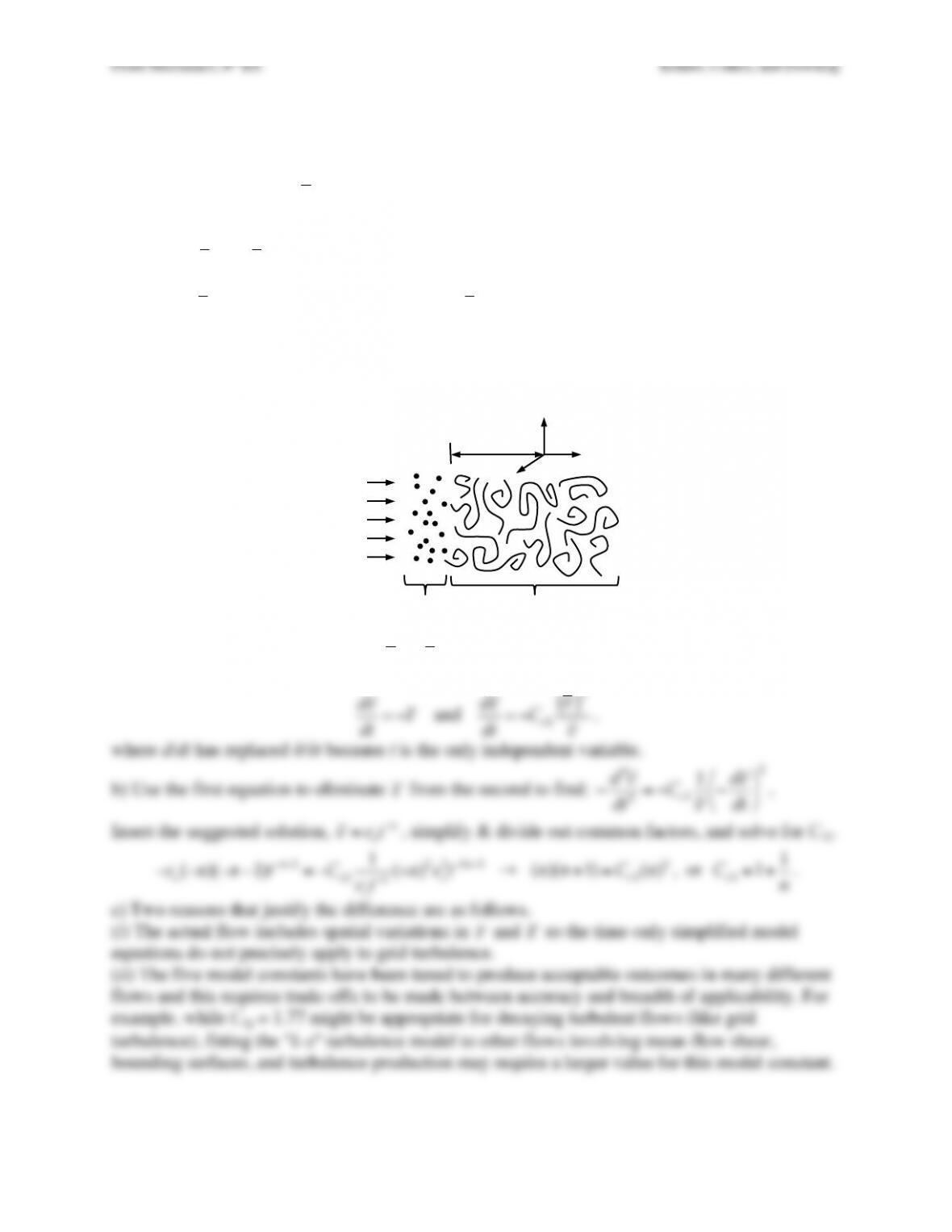
a) Simplify (12.124) and (12.126) for random grid turbulence when Ui = 0.
b) Assume
e(t)
follows a power-law solution,
e=eot−n
, where eo and n are positive constants,
and determine a formula for the model constant C
ε
2 in terms of n.
c) The experimental value of n is approximately 1.3, so the part b) formula then predicts C
ε
2 =
1.77, which is below the standard value (C
ε
2 = 1.92 from Launder & Sharma, 1974). Provide at
least two reasons that justify this discrepancy.
Solution 12.44. a) When Ui = 0 and
e
&
ε
are both functions of time t alone, all the terms with
spatial derivatives (∂/∂xj) drop out. Thus, the simplified model equations are:
de
dt =−
ε
and
d
ε
dt =−C
ε
2
ε
( )
2
e
,
where d/dt has replaced ∂/∂t because t is the only independent variable.
b) Use the first equation to eliminate
ε
from the second to find:
−d2e
ε
2
1
“
#
$%
&
‘
2
e
ε
,
Ut!
random grid!
U!
grid turbulence!
Fluid Mechanics, 6th Ed. Kundu, Cohen, and Dowling
Exercise 12.45. Derive (12.127) from (12.35) with constant density using the definition
equalities in (12.128), (12.129), and (12.131).
Solution 12.45. Start from (12.35) with constant density (
α
= 0):
∂
uiuj
∂
t+Uk
∂
uiuj
∂
xk
+
∂
uiujuk
∂
xk
=−uiuk
∂
Uj
∂
xk
−ujuk
∂
Ui
∂
xk
−1
ρ
ui
∂
p
∂
xj
+uj
∂
p
∂
xi
“
#
$
$
%
&
‘
‘−2
ν∂
ui
∂
xk
∂
uj
∂
xk
+
ν∂
2
∂
xk
2uiuj
Rearrange the terms so that the first four are the same as in (12.127):
∂
uiuj
∂
t+Uk
∂
uiuj
∂
xk
=−uiuk
∂
Uj
∂
xk
−ujuk
∂
Ui
∂
xk
−2
ν∂
ui
∂
xk
∂
uj
∂
xk
−1
ρ
ui
∂
p
∂
xj
+uj
∂
p
∂
xi
“
#
$
$
%
&
‘
‘+
ν∂
2
∂
xk
2uiuj−
∂
uiujuk
∂
xk
The fifth term is
ε
ij as defined by (12.128). The remaining terms on the right may be rewritten to
extract a ∂/∂xk differentiation from everything but the pressure-rate-of-strain tensor.
−1
ρ
ui
∂
p
∂
xj
+uj
∂
p
∂
xi
“
#
$
$
%
&
‘
‘+
ν∂
2
∂
xk
2uiuj−
∂
uiujuk
∂
xk
=−1
ρ
∂
∂
xj
uip−p
∂
ui
∂
xj
+
∂
∂
xi
ujp−p
∂
uj
∂
xi
“
#
$
$
%
&
‘
‘+
∂
∂
xk
ν∂
∂
xk
uiuj−uiujuk
“
#
$%
&
‘
=−1
ρ
∂
∂
xk
uip
δ
jk −p
∂
ui
∂
xj
+
∂
∂
xk
ujp
δ
ik −p
∂
uj
∂
xi
“
#
$
$
%
&
‘
‘+
∂
∂
xk
ν∂
∂
xk
uiuj−uiujuk
“
#
$%
&
‘
=
∂
∂
xk
ν∂
∂
xk
uiuj−uiujuk−uip
ρδ
jk −ujp
ρδ
ik
“
#
$
$
%
&
‘
‘+1
ρ
p
∂
ui
∂
xj
+p
∂
uj
∂
xi
“
#
$
$
%
&
‘
‘
=Mij +Nij
The first equality above follows from the product rule of differentiation and the fact that spatial
differentiation and averaging are independent operations that can be performed in either order.
Thus, the rearranged version of (12.35) for constant density is:
∂
uiuj
∂
t+Uk
∂
uiuj
∂
xk
=−uiuk
∂
Uj
∂
xk
−ujuk
∂
Ui
∂
xk
−
ε
ij +Mij +Nij
,
where (12.129) has been used for Mij and (12.131) has been used for Nij. This final equation is is
(12.127)
Fluid Mechanics, 6th Ed. Kundu, Cohen, and Dowling
Exercise 12.46. Derive (12.132) by taking the divergence of the constant-density Navier-Stokes
momentum equation, computing its average, using the continuity equation, and then subtracting
the averaged equation from the instantaneous equation.
Solution 12.46. Start with the constant density NS-momentum equation with the nonlinear term
written in flux form [see (4.23)]:
∂
!
ui
∂
t+
∂
∂
xj
!
ui!
uj
( )
=−1
ρ
∂
!
p
∂
xi
+
ν∂
2!
ui
∂
xj
∂
xj
,
where as in (12.24) a tilde indicates the full value of a dependent field variable. Take the
Performing the xj-differentiation on the first two term on the right side:
∂
2p
∂
xi
∂
xi
=−
ρ∂
∂
xi
∂
Ui
∂
xj
uj+Ui
∂
uj
∂
xj
+
∂
ui
∂
xj
Uj+ui
∂
Uj
∂
xj
“
#
$
$
%
&
‘
‘−
ρ∂
∂
xi
∂
∂
xj
uiuj−uiuj
( )
.
The second and fourth terms inside the large parentheses are zero for incompressible flow.
Fluid Mechanics, 6th Ed. Kundu, Cohen, and Dowling
Exercise 12.47. Using the Green’s function given in Exercise 12.14 and the properties of
homogeneous turbulence, formally solve (12.132) and then use (12.131) to reach (12.133).
Solution 12.47. From Exercise 12.14, the Green’s function solution of the Poisson equation
∂2p∂xi
2=f(xj)
, is:
p(xj)=−1
4
π
1
(xj−yj)2
all y
∫f(yj)d3y=−1
4
π
1
x−y
all y
∫f(y)d3y
,
where the second form merely involves changes in notation. For the present purposes, the
inhomogeneous term in (12.132) is:
f=−2
ρ∂
Ui
∂
xj
∂
uj
∂
xi
−
ρ∂
∂
xi
∂
∂
xj
uiuj−uiuj
( )
,
thus the formal solution of (12.132) is:
p(x)=−1
4
π
1
x−y
all y
∫−2
ρ∂
Ui
∂
yj
∂
uj
∂
yi
−
ρ∂
∂
yi
∂
∂
yj
uiuj−uiuj
( )
#
$
%
%
&
‘
(
(d3y
.
Using this formal solution, the pressure-rate-of-strain tensor Nij may be written:
Nij ≡p
ρ
∂ui
∂xj
+∂uj
∂xi
#
$
%
%
&
‘
(
(=1
4
π
∂ui
∂xj
1
x−y
all y
∫2
∂
Uk
∂
yl
∂
ul
∂
yk
+
∂
∂
yk
∂
∂
yl
ukul−ukul
( )
#
$
%&
‘
(d3y
1
4
π
∂uj
∂xi
1
x−y
all y
∫2
∂
Uk
∂
yl
∂
ul
∂
yk
+
∂
∂
yk
∂
∂
yl
ukul−ukul
( )
#
$
%&
‘
(d3y.
Combine terms with like integrands:
Fluid Mechanics, 6th Ed. Kundu, Cohen, and Dowling
Exercise 12.48. Turbulence largely governs the mixing and transport of water vapor (and other
gases) in the atmosphere. Such processes can sometimes be assessed by considering the
conservation law (12.34) for a passive scalar.
a) Appropriately simplify (12.34) for turbulence at high Reynolds number that is characterized
by: an outer length scale of L, a large-eddy turnover time of T, and a mass-fraction magnitude of
Yo. In addition, assume that the molecular diffusivity
κ
m is at most as large as
ν
=
µρ
= the
fluid’s kinematic viscosity.
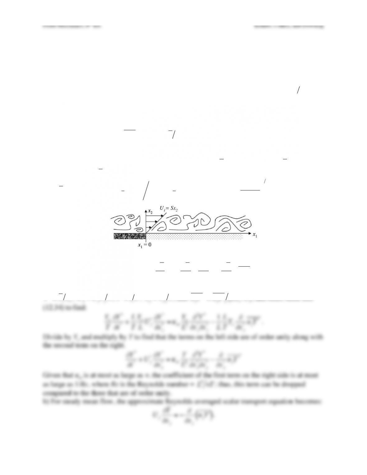
b) Now consider a simple model of how a dry turbulent wind collects moisture as it blows over a
nominally flat water surface (x1 > 0) from a dry surface (x1 < 0). Assume the mean velocity is
steady and has a single component with a linear gradient,
Uj=(Sx2,0,0)
, and use a simple
gradient diffusion model:
−uj#
Y =ΔUL 0,
∂
Y
∂
x2,0
( )
, where ΔU and L are (constant) velocity and
length scales that characterize the turbulent diffusion in this case. This turbulence model allows
the turbulent mean flow to be treated like a laminar flow with a large diffusivity = ΔUL (a
turbulent diffusivity). For the simple boundary conditions:
Y (xj)=0
for x1 < 0,
Y (xj)=1
at x2
= 0 for x1 > 0, and
Y (xj)→0
as
x2→ ∞
, show that
Y (x1,x2,x3)=exp −1
9
ζ
3
( )
ξ
∞
∫d
ζ
exp −1
9
ζ
3
( )
0
∞
∫d
ζ
where
ξ
=x2
S
ΔULx1
$
%
&
‘
(
)
1 3
for x1,x2 > 0.
Solution 12.48. a) Start with (12.34):
∂
Y
∂
t+Uj
∂
Y
∂
xj
=
∂
∂
xj
κ
m
∂
Y
∂
xj
−uj%
Y
&
‘
(
(
)
*
+
+
, but not all the terms
are needed at high Reynolds number. Using the length, time, and mass-fraction scales, set
Y*=Y Yo
,
Uj
*=UjT L
,
t*=t T
,
xj
*=xjL
, and
uj“
Y
*=uj“
Y LYo/T
( )
, and insert these into
(12.34) to find:
Fluid Mechanics, 6th Ed. Kundu, Cohen, and Dowling
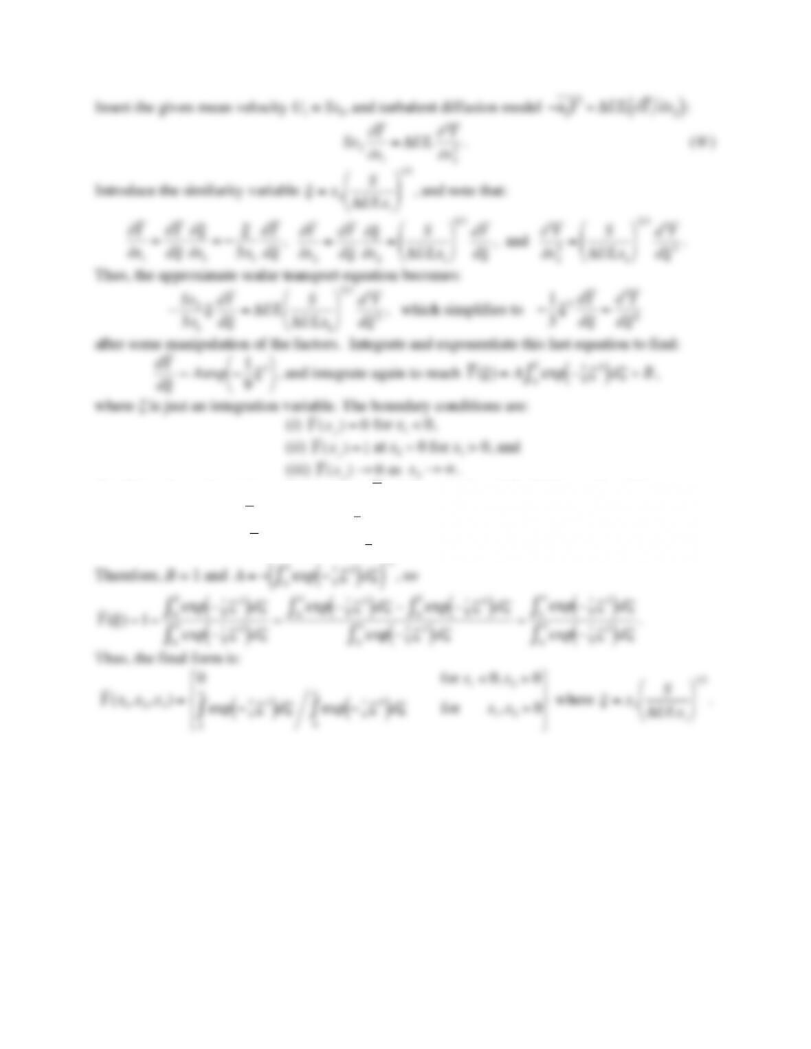
Insert the given mean velocity U1 = Sx2, and turbulent diffusion model
−u2#
Y =ΔUL
∂
Y
∂
x2
( )
:
Condition (i) can be set immediately since
Y =0
is a solution of the field equation (@).
Condition (ii) implies:
Y (0) =Aexp −1
9
ζ
3
( )
d
ζ
0
0
∫+B=1
, or 0+B = 1 for x1 > 0.
Condition (iii) implies:
Y (∞)=Aexp −1
9
ζ
3
( )
d
ζ
0
∞
∫+B=0
, or 0+B = 1 for x1 > 0.
Therefore, B = 1 and
A=−exp −1
9
ζ
3
( )
d
ζ
0
∞
∫
( )
−1
, so
Fluid Mechanics, 6th Ed. Kundu, Cohen, and Dowling
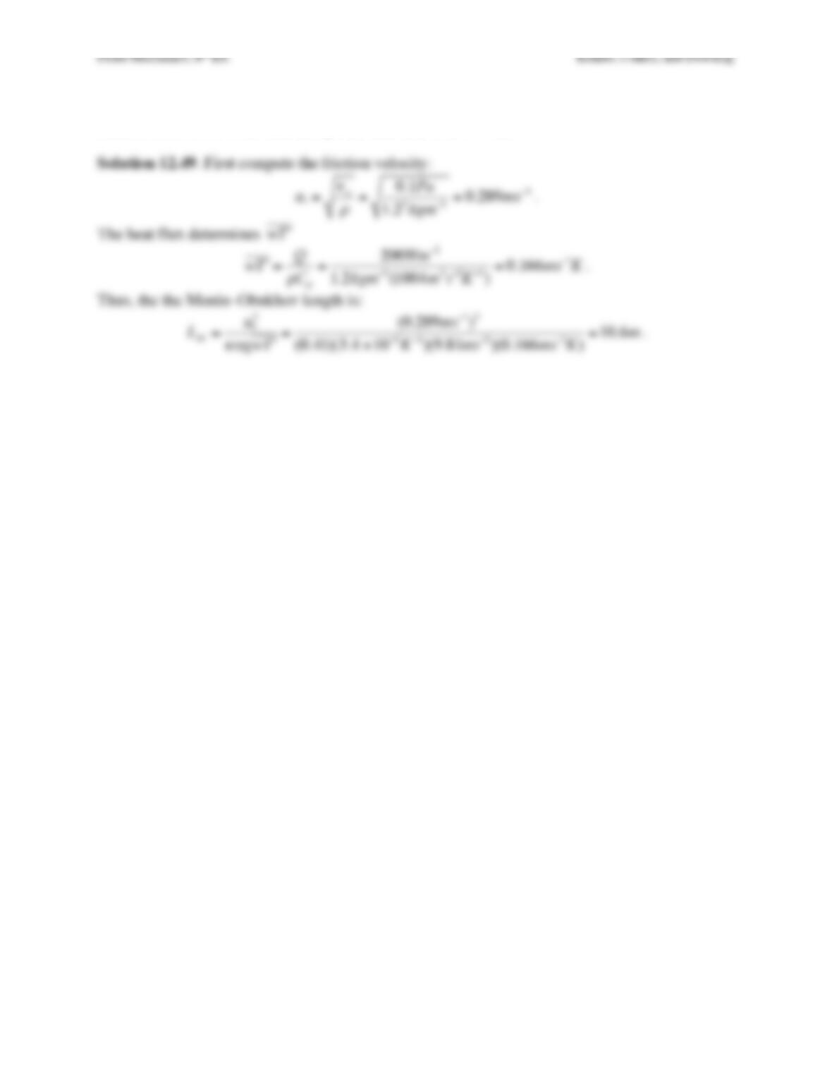
Exercise 12.49. Estimate the Monin–Obukhov length in the atmospheric boundary layer if the
surface stress is 0.1 N/m2 and the upward heat flux is 200 W/m2.
Fluid Mechanics, 6th Ed. Kundu, Cohen, and Dowling
Exercise 12.50. Consider one-dimensional turbulent diffusion of particles issuing from a point
source. Assume a Gaussian Lagrangian correlation function of particle velocity
r(
τ
)=exp −
τ
2tc
2
{ }
,
where tc is a constant. By integrating the correlation function from
τ
= 0 to ∞, find the integral
time scale Λt in terms of tc. Using the Taylor theory, estimate the eddy diffusivity at large times
t/Λt >> 1, given that the rms fluctuating velocity is 1 m/s and tc = 1 s.
Solution 12.50. Start from the definition of the integral time scale:
Λt=r(
τ
)d
τ
0
∞
∫=exp −
τ
2
tc
2
‘
(
)
*
+
,
d
τ
0
∞
∫=exp −
τ
2
tc
2
‘
(
)
*
+
,
d
τ
0
∞
∫=tcexp −
β
2
( )
d
β
0
∞
∫=tc
π
2=0.886tc
.
From (12.129),
DT≅u2Λt=(1ms−1)2⋅0.886(1s)=0.886m2s−1
.