Fluid Mechanics, 6th Ed. Kundu, Cohen, and Dowling
Fluid Mechanics, 6th Ed. Kundu, Cohen, and Dowling
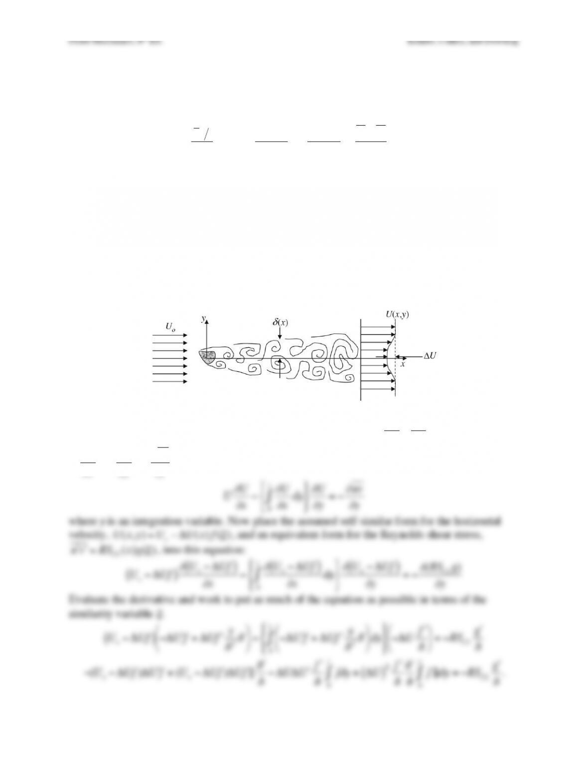
Exercise 12.27. Consider the turbulent wake far from a two-dimensional body placed
perpendicular to the direction of a uniform flow. Using the notation defined in the Figure, the
result of Example 12.5 may be written:
<Begin Equation>
FDl
ρ
Uo
2=
θ
=U(x,y)
Uo
1−U(x,y)
Uo
“
#
$%
&
‘+v2−u2
Uo
2
(
)
*
*
+
,
–
–dy
−∞
+∞
∫
,
</End Equation>
where
θ
is the momentum thickness of the wake flow (a constant), and U(x,y) is the average
horizontal velocity profile a distance x downstream of the body.
a) When ΔU << Uo, find the conditions necessary for a self-similar form for the wake’s velocity
deficit,
U(x,y)=Uo− ΔU(x)f(
ξ
)
, to be valid based on the equation above and the steady two-
dimensional continuity and boundary-layer RANS equations. Here,
ξ
= y/
δ
(x) and
δ
is the
transverse length scale of the wake.
b) Determine how ΔU and
δ
must depend on x in the self-similar region. State your results in
appropriate dimensionless form using
θ
and Uo as appropriate.
Solution 12.27. a) The steady boundary layer RANS equations are:
∂
U
∂
x+
∂
V
∂
y=0
, and
U
∂
U
∂
x+V
∂
U
∂
y=−
∂
uv
∂
y
. First combine the momentum & continuity equations to eliminate V:
U
∂
U
∂
x−
∂
U
∂
xdy
0
y
∫
%
&
‘
(
)
*
∂
U
∂
y=−
∂
uv
∂
y
where y is an integration variable. Now place the assumed self-similar form for the horizontal
velocity,
U(x,y)=Uo− ΔU(x)f(
ξ
)
, and an equivalent form for the Reynolds shear stress,
“
u “
v =RSCL (x)g(
ξ
)
, into this equation:
Uo− ΔUf
( )
∂
Uo− ΔUf
( )
∂
x−
∂
Uo− ΔUf
( )
∂
xdy
0
y
∫
&
‘
(
)
*
+
∂
Uo− ΔUf
( )
∂
y=−
∂
(RSCL g)
∂
y
Evaluate the derivative and work to put as much of the equation as possible in terms of the
similarity variable
ξ
.
Uo− ΔUf
( )
−Δ $
U f+ΔU$
f y
δ
2$
δ
&
‘
( )
*
+ − −Δ $
U f+ΔU$
f y
δ
2$
δ
&
‘
( )
*
+
dy
0
y
∫
–
.
/
0
1
2 −ΔU$
f
δ
&
‘
( )
*
+ =−RSCL
$
g
δ
−(Uo− ΔUf )Δ$
U f+(Uo− ΔUf )ΔU$
f
ξ
$
δ
δ
− ΔUΔ$
U $
f
δ
fdy
0
y
∫+ΔU
( )
2$
f
δ
$
δ
δ
$
f
ξ
dy
0
y
∫=−RSCL
$
g
δ
.
Fluid Mechanics, 6th Ed. Kundu, Cohen, and Dowling
Fluid Mechanics, 6th Ed. Kundu, Cohen, and Dowling
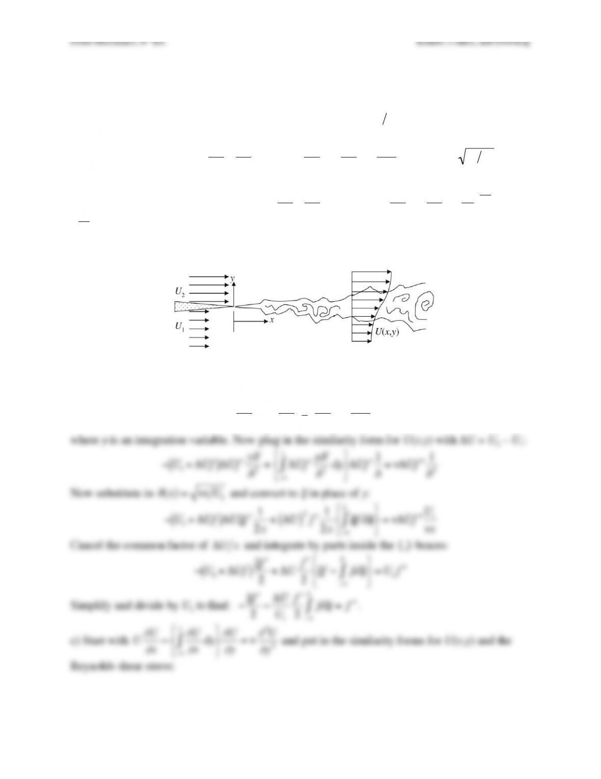
Exercise 12.28. Consider the two-dimensional shear layer that forms between two steady
streams with flow speed U2 above and U1 below y = 0, that meet at x = 0, as shown. Assume a
self-similar form for the average horizontal velocity:
U(x,y)=U1+(U2−U1)f(
ξ
)
with
ξ
=y
δ
(x)
.
a) What are the boundary conditions on f(
ξ
) as y → ±∞?
b) If the flow is laminar, use
∂
U
∂
x+
∂
V
∂
y=0
and
U
∂
U
∂
x+V
∂
U
∂
y=
ν∂
2U
∂
y2
with
δ
(x)=
ν
x U1
to
obtain single equation for f(
ξ
). There is no need to solve this equation.
c) If the flow is turbulent, use:
∂
U
∂
x+
∂
V
∂
y=0
and
U
∂
U
∂
x+V
∂
U
∂
y=−
∂
∂
yuv
( )
with
−uv =U2−U1
( )
2g(
ξ
)
to obtain a single equation involving f and g. Determine how
δ
must
depend on x for the flow to be self-similar.
d) Does the laminar or the turbulent mixing layer grow more quickly as x increases?
Solution 12.28. a) As y → –∞, f(
ξ
)→ 0; and as y → +∞, f(
ξ
)→ 1.
b) First combine the equations to eliminate V:
U
∂
U
∂
x−
∂
U
∂
xdy
−∞
y
∫
&
‘
(
)
*
+
∂
U
∂
y=
ν∂
2U
∂
y2
.
where y is an integration variable. Now plug in the similarity form for U(x,y) with ΔU = U2 – U1:
U
∂
U
∂
x−
∂
U
∂
xdy
−∞
y
∫
∂
U
∂
y=
ν∂
∂
Reynolds shear stress:
Fluid Mechanics, 6th Ed. Kundu, Cohen, and Dowling
Fluid Mechanics, 6th Ed. Kundu, Cohen, and Dowling
Exercise 12.29. Consider an orifice of diameter d that emits an incompressible fluid of density
ρ
o
at speed Uo into an infinite half space of fluid with density
ρ
∞. With gravity acting and
ρ
∞ >
ρ
o, the
orifice fluid rises, mixes with the ambient fluid, and forms a buoyant plume with a diameter D(z)
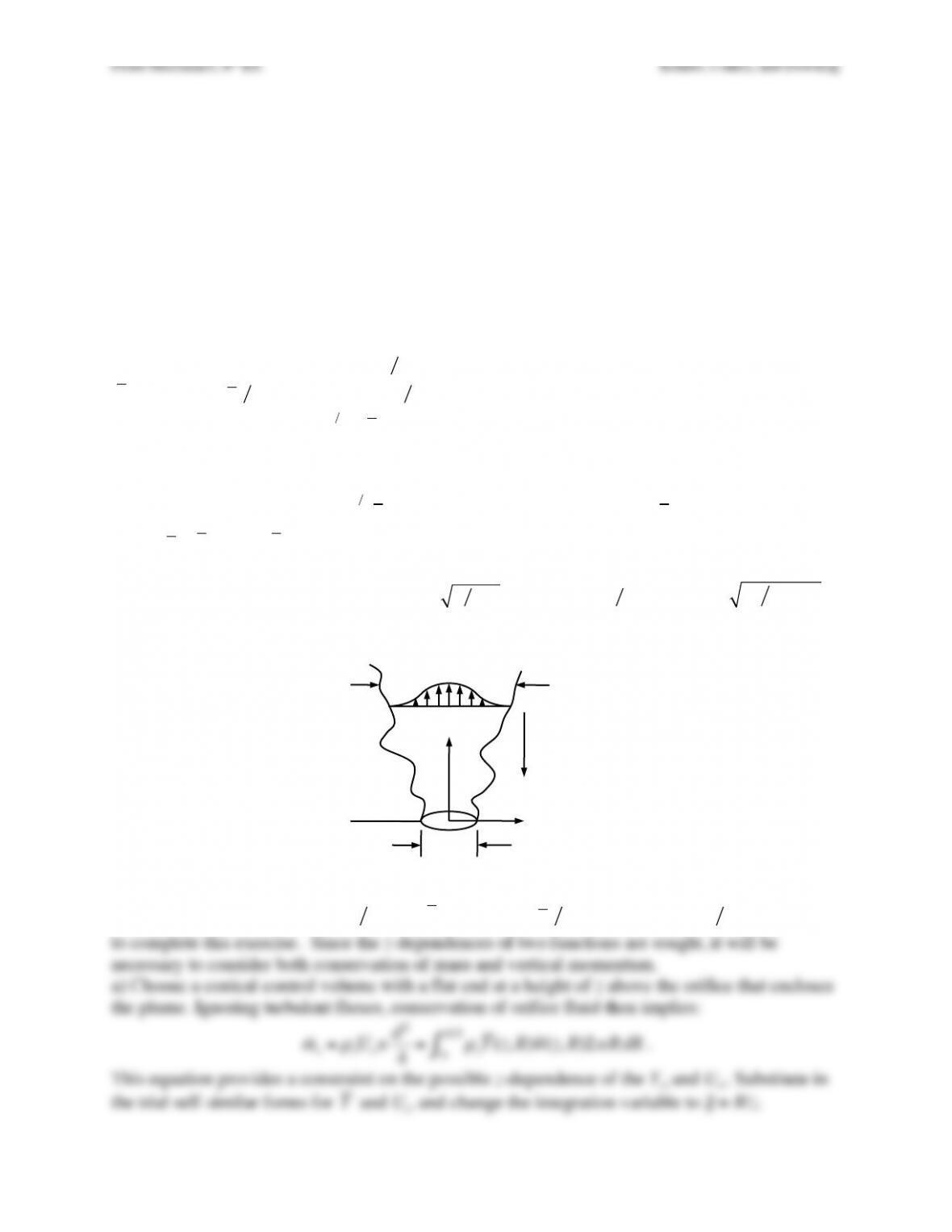
that grows with increasing height above the orifice. Assuming that the plume is turbulent and
self-similar in the far-field (z >> d), determine how the plume diameter D, the mean centerline
velocity Ucl, and the mean centerline mass fraction of orifice fluid Ycl depend on the vertical
coordinate z via the steps suggested below. Ignore the initial momentum of the orifice fluid. Use
both dimensional and control-volume analysis as necessary. Ignore streamwise turbulent fluxes
to simplify your work. Assume uniform flow from the orifice.
a) Place a stationary cylindrical control volume around the plume with circular control surfaces
that slice through the plume at its origin and at height z. Use similarity forms for the average
vertical velocity
Uz(z,R)=Ucl (z)f R z
( )
and nozzle fluid mass fraction
Y(z,R)=(
ρ
∞−
ρ
) (
ρ
∞−
ρ
o)=Ycl (z)h R z
( )
to conserve the flux of nozzle fluid in the plume, and
find:
mo=
ρ
oUodA
source
∫=
ρ
oY(z,R)Uz(z,R)2
π
R dR
0
D2
∫
.
b) Conserve vertical momentum using the same control volume assuming that all entrained fluid
enters with negligible vertical momentum, to determine:
−
ρ
oUo
2dA
source
∫+
ρ
(z,R)Uz
2(z,R)2
π
R dR
0
D2
∫=g
ρ
∞−
ρ
(z,R)
[ ]
dV
volume
∫
,
where
ρ
=Y
ρ
o+(1−Y)
ρ
∞
.
c) Ignore the source momentum flux, assume z is large enough so that YCL << 1, and use the
results of parts a) and b) to find:
Ucl (z)=C1.B
ρ
∞z
3
and
(
ρ
∞−
ρ
o)
ρ
∞
( )
Ycl (z)=C2B2g3
ρ
∞
2z5
3
,
where C1 and C2 are dimensionless constants, and
B=(
ρ
∞−
ρ
o)gUodA
source
∫
.
Solution 12.29. Use the similarity forms provided,
Uz(z,R)=Ucl (z)f R z
( )
and
Y(z,R)=(
ρ
∞−
ρ
) (
ρ
∞−
ρ
o)=Ycl (z)h R z
( )
to complete this exercise. Since the z-dependences of two functions are sought, it will be
z!
R!
ρ
∞”
g!
D(z)“
UCL(z)f(R/z)“
d!
Fluid Mechanics, 6th Ed. Kundu, Cohen, and Dowling
−
ρ
oUo
source
∫dA +
ρ
(z,R)wUz
π
R dR
0
∫=−g
ρ
(z,R)dV
volume
∫−Pn⋅ez
( )
surface
∫dA
.
c) The first integral on the right results from the gravitational body force, and the second term is
the pressure integral. The pressure on the conical control surface will be the hydrostatic pressure:
P = Po –
ρ
∞gz. If we assume that the flow is basically upward within the plume, the radial
momentum equation can be used to find ∂P/∂r ≈ 0 so the foregoing pressure equation can be
used at any radial location. So, use the static pressure relationship and Gauss’ Theorem to
Fluid Mechanics, 6th Ed. Kundu, Cohen, and Dowling
Fluid Mechanics, 6th Ed. Kundu, Cohen, and Dowling
Exercise 12.30. Laminar and turbulent boundary layer skin friction are very different. Consider
skin friction correlations from zero-pressure-gradient (ZPG) boundary layer flow over a flat plate
placed parallel to the flow.
Laminar boundary layer:
Cf=
τ
0
1
2
ρ
U2=0.664
Rex
(Blasuis boundary layer)
Turbulent boundary layer: (see correlations in §12.9)
Create a table of computed results at Rex = Ux/
ν
= 104, 105, 106, 107, 108, and 109 for the laminar
and turbulent skin friction coefficients, and the friction force acting on 1.0 m2 plate surface in
sea-level air at 100 m/s and in water at 20 m/s assuming laminar and turbulent flow.
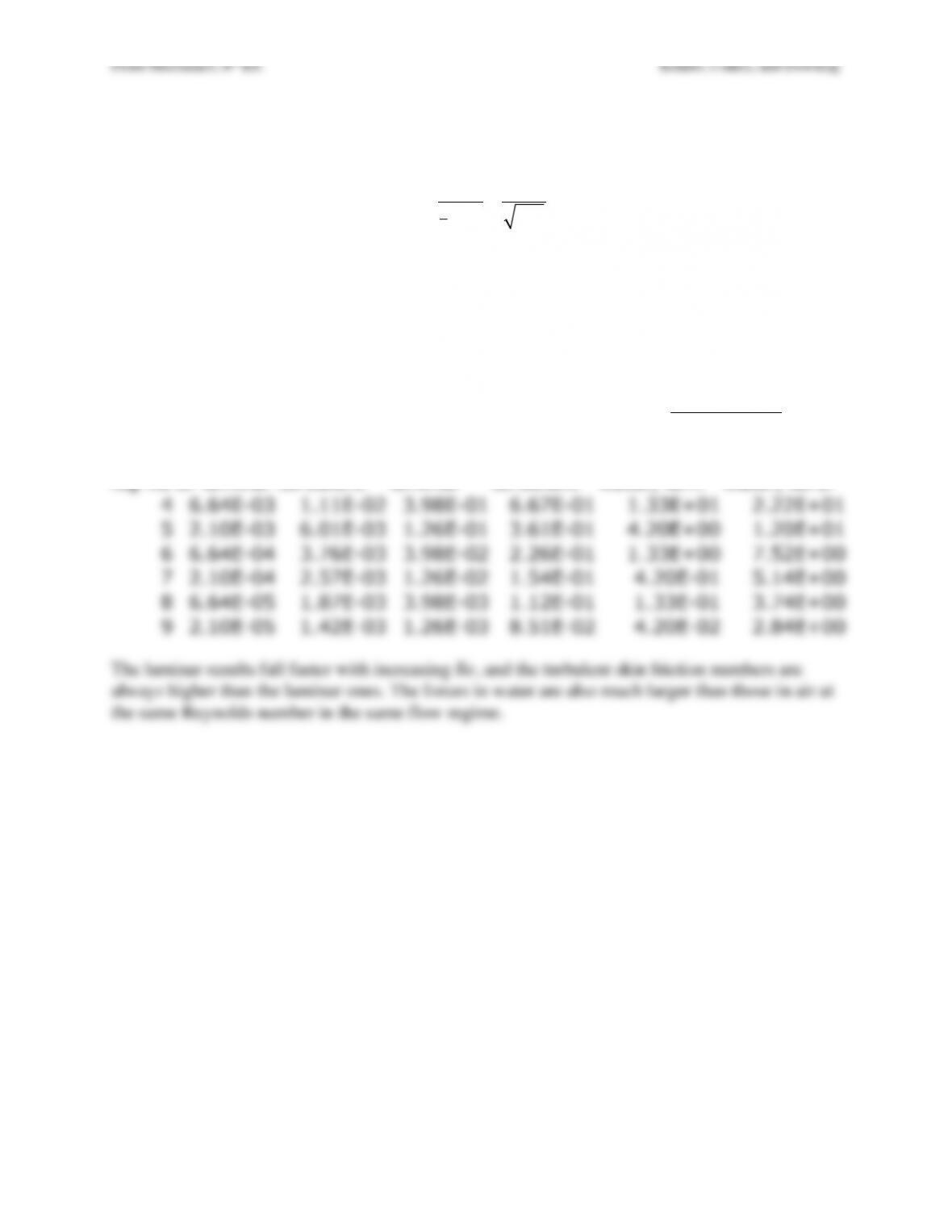
Solution 12.30. Merely calculate and tabulate results for air:
ρ
= 1.2 kg/m3 &
ν
= 1.5×10⁻⁵ m2/s,
and for water:
ρ
= 103 kg/m3 &
ν
= 10–6 m2/s. The forces below are in Newtons, and the
turbulent skin friction numbers were obtained from White’s formula:
Cf≅0.455
ln 0.06Rex
( )
[ ]
2
.
log Re
Cf laminar
Cf
turbulent
Force, air,
laminar
Force, air,
turbulent
Force,
water, lam.
Force,
water, turb.
4
6.64E–03
1.11E–02
3.98E–01
6.67E–01
1.33E+01
2.22E+01
5
2.10E–03
6.01E–03
1.26E–01
3.61E–01
4.20E+00
1.20E+01
6
6.64E–04
3.76E–03
3.98E–02
2.26E–01
1.33E+00
7.52E+00
7
2.10E–04
2.57E–03
1.26E–02
1.54E–01
4.20E–01
5.14E+00
8
6.64E–05
1.87E–03
3.98E–03
1.12E–01
1.33E–01
3.74E+00
9
2.10E–05
1.42E–03
1.26E–03
8.51E–02
4.20E–02
2.84E+00
The laminar results fall faster with increasing Re, and the turbulent skin friction numbers are
always higher than the laminar ones. The forces in water are also much larger than those in air at
the same Reynolds number in the same flow regime.
Fluid Mechanics, 6th Ed. Kundu, Cohen, and Dowling
Exercise 12.31. Derive the following logarithmic velocity profile for a smooth wall:
U+=1
κ
( )
ln y++5.0
by starting from
U=u*
κ
( )
ln y++const.
and matching the profile to the
edge of the viscous sublayer assuming the viscous sublayer ends at y = 10.7 v/u*.
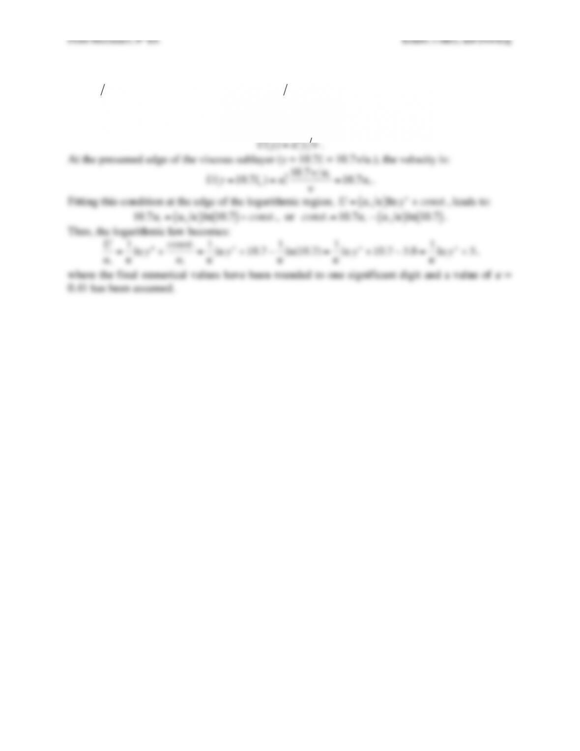
Solution 12.31. In the viscous sublayer the velocity profile is linear:
U(y)=u*
2y
ν
.
At the presumed edge of the viscous sublayer (y = 10.7l
ν
= 10.7
ν
/u*), the velocity is:
U(y=10.7l
ν
)=u*
210.7
ν
u*
ν
=10.7u*
.
Fitting this condition at the edge of the logarithmic region,
U=u*
κ
( )
ln y++const.
, leads to:
Fluid Mechanics, 6th Ed. Kundu, Cohen, and Dowling
Exercise 12.32. Derive the log-law for the mean flow profile in a zero-pressure gradient (ZPG)
flat plate turbulent boundary layer (TBL) through the following mathematical and dimensional
arguments.
a) Start with the law of the wall,
U u*=fyu*
ν
( )
or
U+=f(y+)
, for the near-wall region of the
boundary layer, and the defect law for the outer region,
Ue−U
u*
=Fy
δ
$
%
& ‘
(
)
. These formulae must
overlap when y+ → +∞ and y/
δ
→ 0. In this matching or overlap region, set U and
∂
U
∂
y
from
both formula equal to get two equations involving f and F.
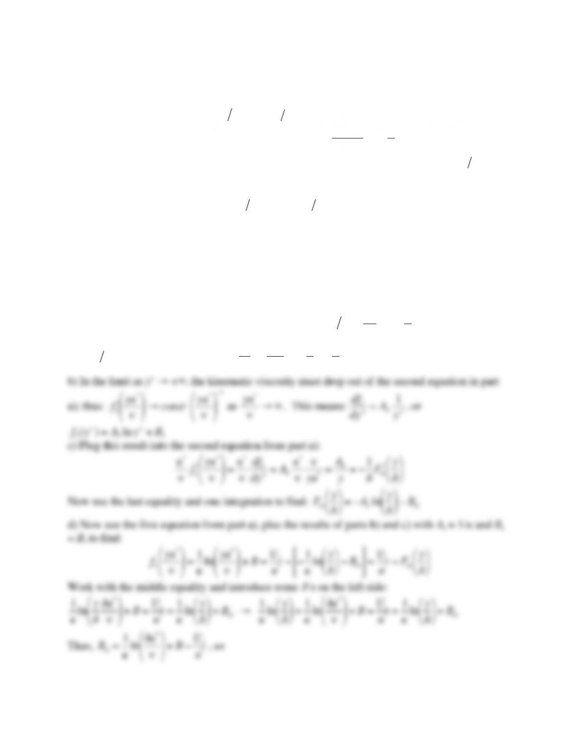
b) In the limit as y+ → +∞, the kinematic viscosity must drop out of the equation that includes
df/dy+. Use this fact, to show that
U u*=AIln yu*
ν
( )
+BI
as y+ → +∞ where AI and BI are
constants for the near-wall or inner boundary layer scaling.
c) Use the result of part b) to determine
F(
ξ
)=−AIln
ξ
( )
−BO
where
ξ
= y/
δ
, and AI and BO are
constants for the wake flow or outer boundary layer scaling.
d) It is traditional to set AI = 1/
κ
, and to keep BI but to drop its subscript. Using these new
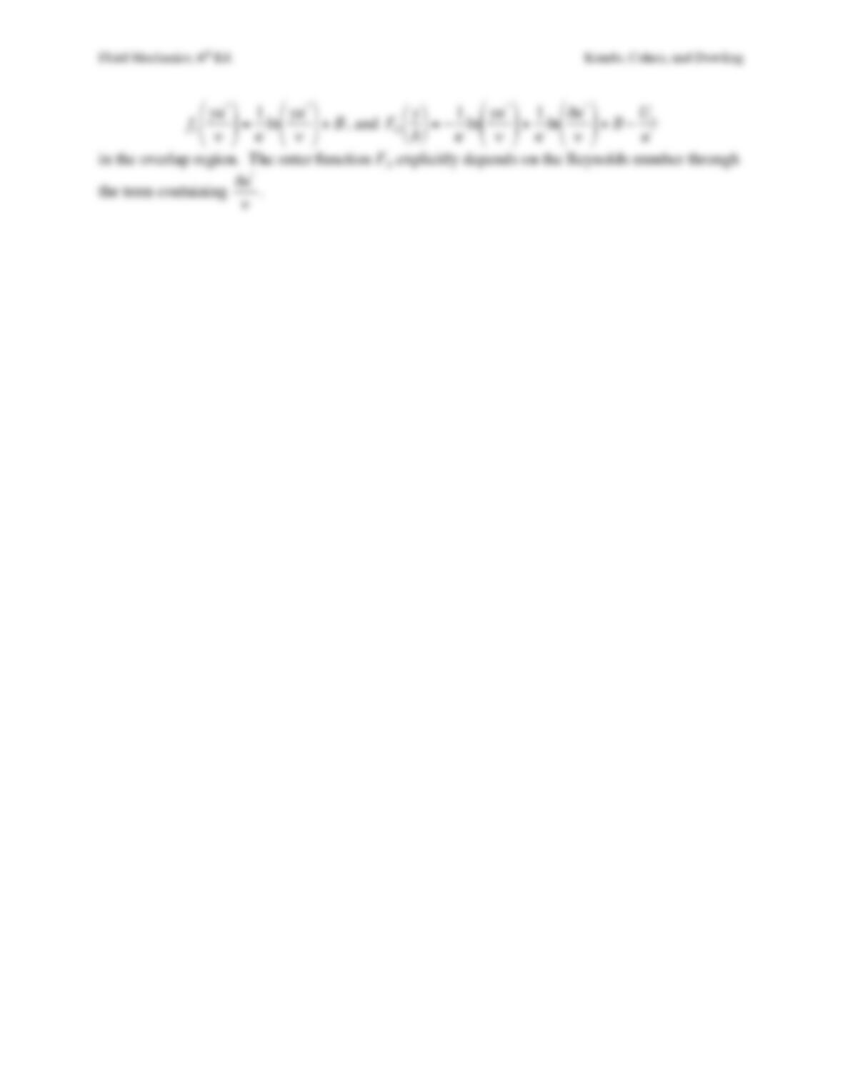
requirements determine the two functions, fI and FO, in the matching region. Which function
explicitly depends on the Reynolds number of the flow?
Solution 12.32. a) Set U from both formulae equal:
fIyu*
ν
( )
=Ue
u*−FO
y
δ
%
&
‘ (
)
*
.
Set
∂
U
∂
y
from both formula equal:
u*
ν
#
f
I
yu*
ν
$
%
&
‘
(
) =−1
δ
#
F
O
y
δ
$
%
& ‘
(
)
.
b) In the limit as y+ → +∞, the kinematic viscosity must drop out of the second equation in part
Fluid Mechanics, 6th Ed. Kundu, Cohen, and Dowling
Fluid Mechanics, 6th Ed. Kundu, Cohen, and Dowling
Exercise 12.33. For zero pressure gradient, the Von Karman boundary layer integral equation
simplifies to Cf = 2d
θ
/dx. Use this fact, and (12.90) to determine Cf and numerically compare this
result to Cf obtained from (12.93). Do the results match well for 106 < Rex < 109? What
difference does the choice of log-law constants make? Consider (
κ
,B) pairs representative of the
nominal modern values for pipes (0.41, 5.2) and boundary layers (0.38, 4.2).
Solution 12.33. Compute the skin friction by differentiating the momentum thickness correlation
(12.90):
Cf=2d
θ
dx =2d
dx
0.016xUex
ν
!
“
#$
%
&
−0.15
(
)
*
*
+
,
–
–=0.032 0.85
( )
Uex
ν
!
“
#$
%
&
−0.15
=0.0272 Rex
−0.15
.
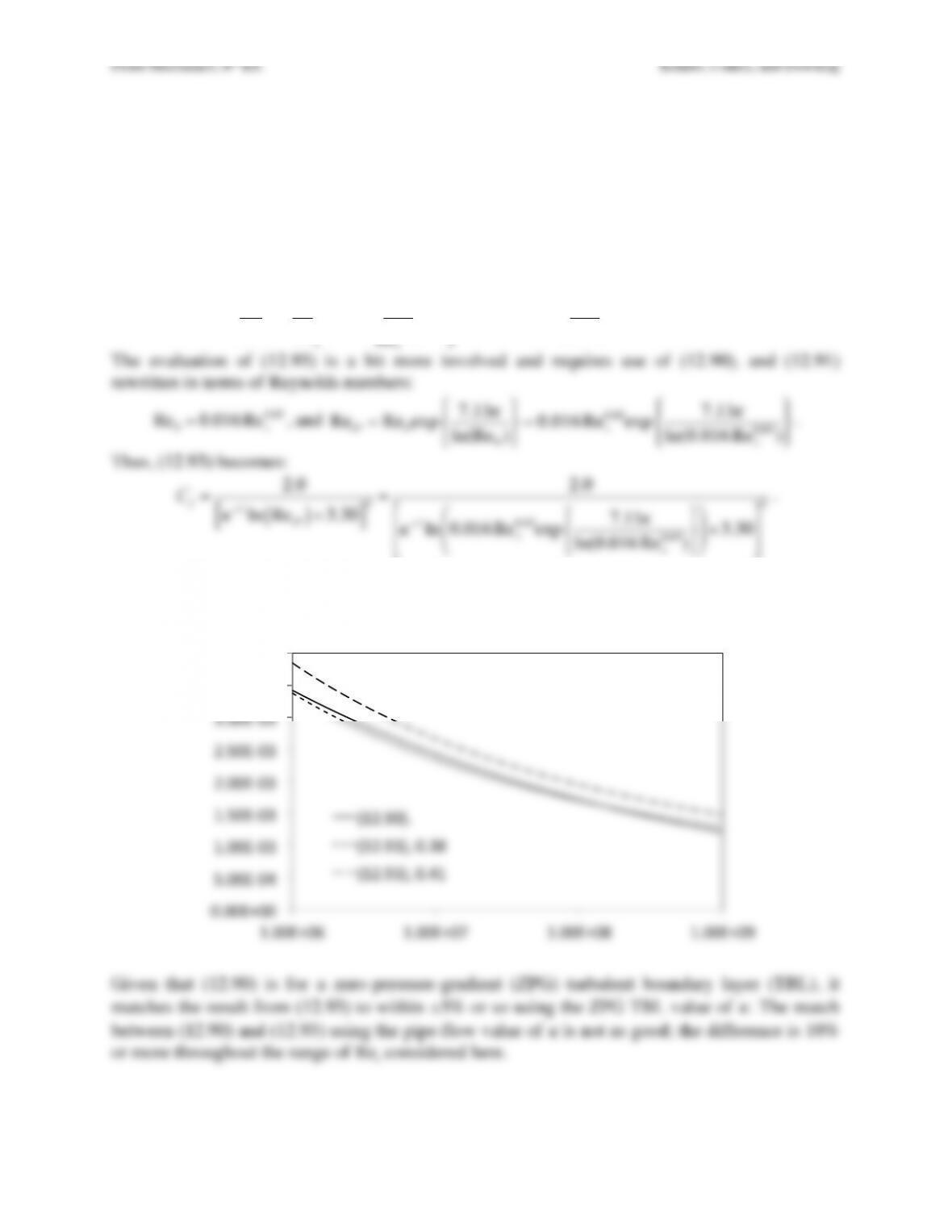
The evaluation of (12.93) is a bit more involved and requires use of (12.90), and (12.91)
(
+
–
0
#
2
%
3
The constant B doesn’t matter, but
κ
does enter the formulation for Cf. For clarity, the
comparison should be made graphically.
matches the result from (12.93) to within ±5% or so using the ZPG TBL value of
κ
. The match
between (12.90) and (12.93) using the pipe-flow value of
κ
is not as good; the difference is 10%
or more throughout the range of Rex considered here.
0.00E+00%
5.00E’04%
1.00E’03%
1.50E’03%
2.00E’03%
2.50E’03%
3.00E’03%
3.50E’03%
4.00E’03%
1.00E+06% 1.00E+07% 1.00E+08% 1.00E+09%
(12.90).%
(12.93),%0.38%
(12.93),%0.41%
Cf
Rex
Fluid Mechanics, 6th Ed. Kundu, Cohen, and Dowling
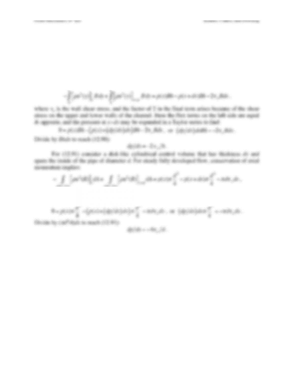
Exercise 12.34. Prove (12.90) and (12.91) by considering a stationary control volume that
resides inside the channel or pipe and has stream-normal control surfaces separated by a distance
dx and stream-parallel surfaces that coincide with the wall or walls that confine the flow.
Solution 12.34. The two calculations are nearly the same.
For (12.90) consider a slab-like control volume that has thickness dx in the stream-wise
direction, width B perpendicular to the mean flow, and height h that spans the inside of the
channel. For steady fully developed flow, conservation of axial momentum implies:
−
ρ
u2(y)
“
#$
%xB dy
0
h
∫+
ρ
u2(y)
“
#$
%x+dx B dy
0
h
∫=p(x)Bh −p(x+dx)Bh −2
τ
wBdx
,
where
τ
w is the wall shear stress, and the factor of 2 in the final term arises because of the shear
stress on the upper and lower walls of the channel. Here the flux terms on the left side are equal
& opposite, and the pressure at x+dx may be expanded in a Taylor series to find:
0=p(x)Bh −p(x)+dp dx
( )
dx
( )
Bh −2
τ
wBdx
, or
dp dx
( )
dxBh =−2
τ
wBdx
.
Divide by Bhdx to reach (12.90):
dp dx =−2
τ
wh
.
For (12.91) consider a disk-like cylindrical control volume that has thickness dx and
spans the inside of the pipe of diameter d. For steady fully developed flow, conservation of axial
momentum implies:
−
ρ
u2(R)
“
#$
%x
pipe area
∫dA +
ρ
u2(R)
“
#$
%x+dx
pipe area
∫dA =p(x)
π
d
4
2
−p(x+dx)
π
d
4
2
−
π
d
τ
wdx
,
where
τ
o is the wall shear stress. Here again, the flux terms on the left side are equal & opposite,
and the pressure at x+dx may be expanded in a Taylor series to find:
0=p(x)
π
d
4
2
−p(x)+dp dx
( )
dx
( )
π
d
4
2
−
π
d
τ
wdx
, or
dp dx
( )
dx
π
d
4
2
=−
π
d
τ
wdx
.
Divide by (
π
d2/4)dx to reach (12.91):
dp dx =−4
τ
wd
.
Fluid Mechanics, 6th Ed. Kundu, Cohen, and Dowling
Exercise 12.35. The log-law occurs in turbulent channel, pipe, or boundary layer flows and
should be absent in laminar flows in the same geometries. The extent of the log-law is governed
by Re
τ
=
δ
+ =
δ
/l
ν
=
δ
u*/
ν
, where
δ
is the channel half-height (h/2), pipe radius (d/2), or full
boundary-layer thickness, as appropriate for each flow geometry.
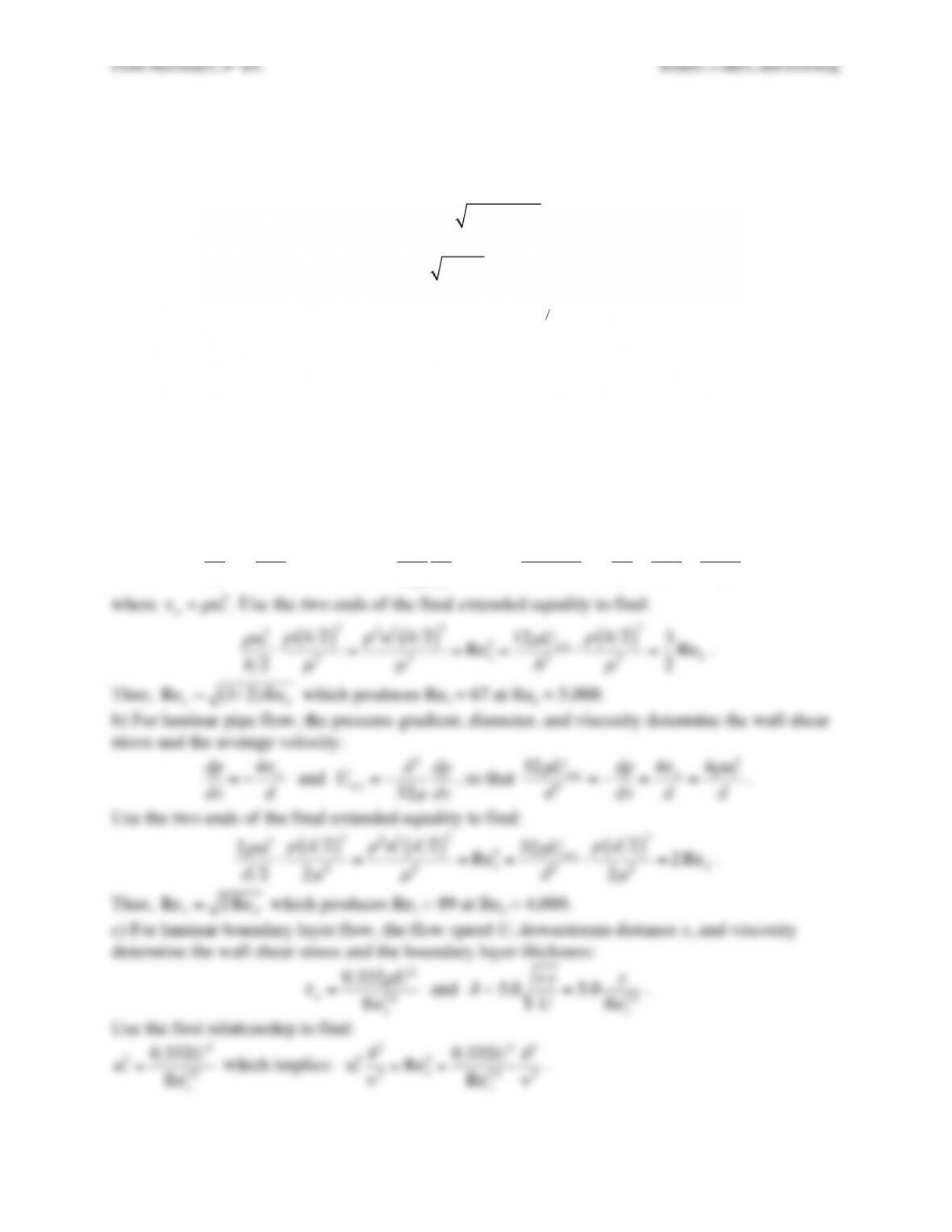
a) For laminar channel flow, show that
Re
τ
=(3 / 2)Reh
, and compute Re
τ
at an approximate
transition Reynolds number of Reh ~ 3,000.
b) For laminar pipe flow, show that
Re
τ
=2 Red
, and compute Re
τ
at an approximate transition
Reynolds number of Red ~ 4,000.
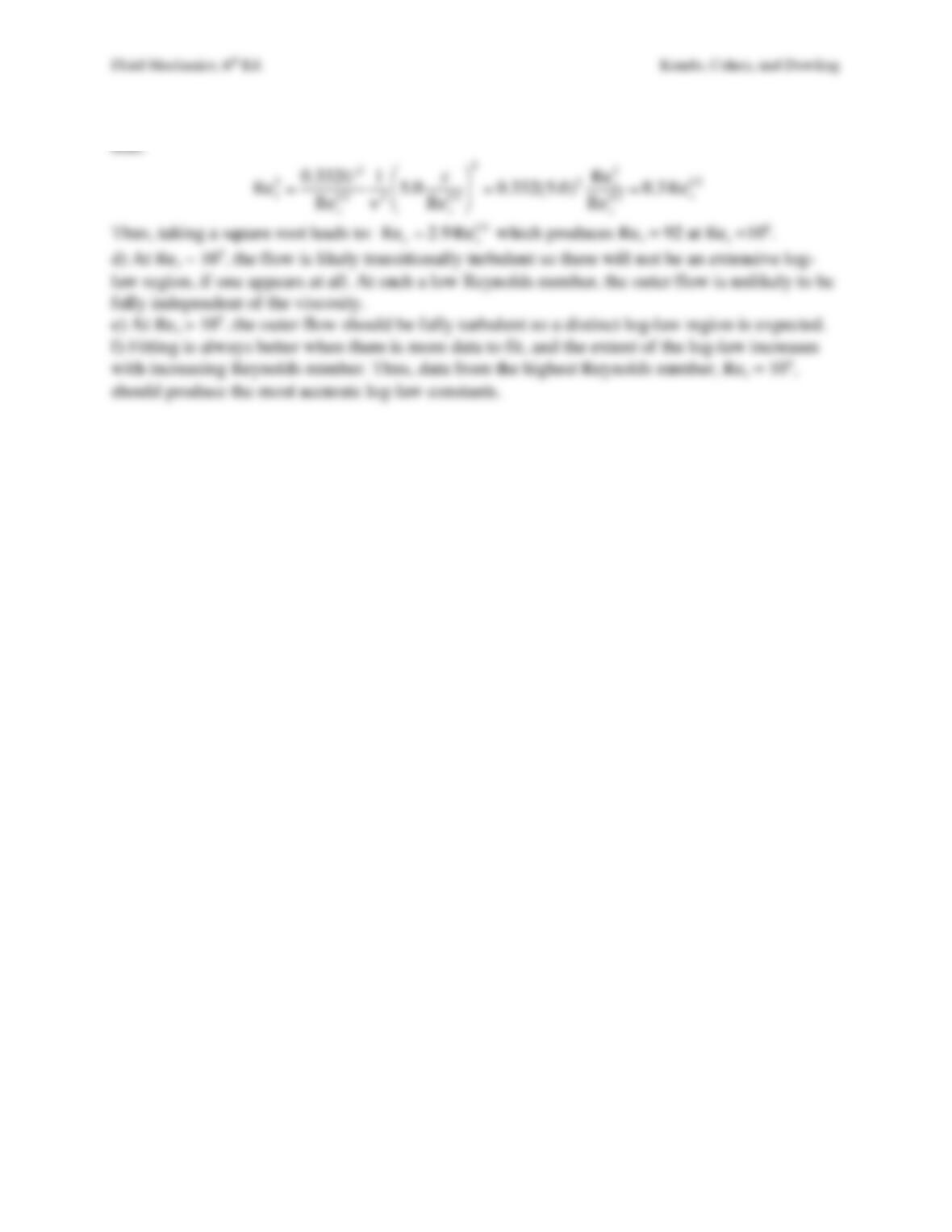
c) For the Blasius boundary layer, show that
Re
τ
≅2.9 Rex
1 4
, and compute Re
τ
at a transition
Reynolds number of Rex ~ 106.
d) If mean profile measurements are made in a wall-bounded turbulent flow at Re
τ
~ 102, do you
expect the profiles to display the log-law? Why or why not?
e) Repeat part d) when Re
τ
> 103.
f) The log-law constants (
κ
and B) are determined from fitting (12.88) to experimental data. At
which Re
τ
are
κ
and B most likely to be accurately determined: 102, 103, or 104?
Solution 12.35. a) For laminar channel flow, the pressure gradient, channel height, and viscosity
determine the wall shear stress and the average velocity:
dp
dx =−2
τ
w
h
and
Uave =−h2
12
µ
dp
dx
, so that
12
µ
Uave
h2=−dp
dx =2
τ
w
h=2
ρ
u*
2
h
.
where
τ
w=
ρ
u*
2
. Use the two ends of the final extended equality to find:
Re
τ
=(3 / 2)Reh
Fluid Mechanics, 6th Ed. Kundu, Cohen, and Dowling
Now use the relationship for the overall-boundary layer thickness
δ
to eliminate
δ
on the right
side.
Fluid Mechanics, 6th Ed. Kundu, Cohen, and Dowling
Exercise 12.36. A horizontal smooth pipe 20 cm in diameter carries water at a temperature of 20
°C. The drop of pressure is dp/dx = –8 N/m2 per meter. Assuming turbulent flow, verify that the
thickness of the viscous sublayer is ≈ 0.25 mm. [Hint: Use dp/dx as given by (12.97) to find
τ
w =
0.4 N/m2, and therefore u* =0.02 m/s.]
Solution 12.36. From (12.96), ∂p/∂x = –4
τ
w/d, therefore:
τ
w=−d
4
∂
p
∂
x=−(0.2m)
4(−8Pa /m)=0.4Pa
, so
u*=
τ
w
ρ
=0.4Pa
103kgm−3=0.02ms−1
.
From Section 12.9, the viscous sublayer thickness is:
5l
ν
=5
ν
u*
( )
=5(1.0 ×10⁻⁶m2s−10.02ms−1)=2.5 ×10⁻⁴m=0.25mm
.