Unlock document.
This document is partially blurred.
Unlock all pages and 1 million more documents.
Get Access
Fluid Mechanics, 6th Ed. Kundu, Cohen, and Dowling
Exercise 12.16. Derive the RANS transport equation for the Reynolds stress correlation (12.35)
via the following steps.
a) By subtracting (12.30) from (4.86), show that the instantaneous momentum equation for the
fluctuating turbulent velocity ui is:
∂
ui
∂
t+uk
∂
Ui
∂
xk
+Uk
∂
ui
∂
xk
+uk
∂
ui
∂
xk
=−1
ρ
0
∂
p
∂
xi
+
ν∂
2ui
∂
xk
2+g
α
'
T
δ
i3+
∂
∂
xk
uiuk
.
b) Show that:
ui
Du j
Dt +uj
Dui
Dt =
∂
∂
tuiuj
( )
+Uk
∂
∂
xk
uiuj
( )
+
∂
∂
xk
uiujuk
( )
.
c) Combine and simplify the results of parts a) and b) to reach (12.35)
Solution 12.16. a) Start from (4.86):
∂
˜
u
i
∂
t+
∂
∂
xj
˜
u
j˜
u
i
( )
=−1
ρ
0
∂
˜
p
∂
xi
−g1−
α
˜
T −T0
( )
[ ]
δ
i3+
ν∂
2˜
u
i
∂
xj
2
,
and insert the Reynolds decompositions (12.24) to find:
∂
∂
tUi+ui
( )
+
∂
∂
xj
(Uj+uj)(Ui+ui)
( )
=−1
ρ
0
∂
∂
xi
(P+p)−g1−
α
T +&
T −T0
( )
[ ]
δ
i3+
ν∂
2
∂
xj
2Ui+ui
( )
,
and subtract (12.30),
∂
Ui
∂
t+Uj
∂
Ui
∂
xj
=−1
ρ
0
∂
P
∂
xi
−g1−
α
T −T0
( )
[ ]
δ
i3+1
ρ
0
∂
∂
xj
∂
Ui
∂
xj
−
ρ
0uiuj
'
(
)
)
*
+
,
,
,
to reach:
∂
ui
∂
t+
∂
∂
xj
ujUi+Ujui+ujui
( )
=−1
ρ
0
∂
p
∂
xi
+g
α
&
T
δ
i3+
ν∂
2ui
∂
xj
2+
∂
∂
xj
uiuj
.
Now use the fact that ∂Uj/∂xj = 0 and ∂uj/∂xj = 0, and switch the summed-over index from
"j" to "k".
∂
ui
∂
t+uk
∂
Ui
∂
xk
+Uk
∂
ui
∂
xk
+uk
∂
ui
∂
xk
=−1
ρ
0
∂
p
∂
xi
+g
α
&
T
δ
i3+
ν∂
2ui
∂
xk
2+
∂
∂
xk
uiuk
.
b) Use "k" as a subscript to denote the dot product within the fluid particle acceleration,
D
Dt =
∂
∂
t+˜
u
k
∂
∂
xk
,
so that:
ui
Du j
Dt +uj
Dui
Dt =ui
∂
uj
∂
t+ui˜
u
k
∂
uj
∂
xk
+uj
∂
ui
∂
t+uj˜
u
k
∂
ui
∂
xk
=
∂
∂
tuiuj
( )
+˜
u
k
∂
∂
xk
uiuj
( )
=
∂
∂
tuiuj
( )
+Uk+uk
( )
∂
∂
xk
uiuj
( )
=
∂
∂
tuiuj
( )
+Uk
∂
∂
xk
uiuj
( )
+uk
∂
∂
xk
uiuj
( )
=
∂
∂
tuiuj
( )
+Uk
∂
∂
xk
uiuj
( )
+
∂
∂
xk
uiujuk
( )
where the final equality follows because ∂uk/∂xk = 0.
c) The result of part a) can be written:
Dui
Dt +uk
∂
Ui
∂
xk
=−1
ρ
0
∂
p
∂
xi
+g
α
&
T
δ
i3+
ν∂
2ui
∂
xk
2+
∂
∂
xk
uiuk
.
Use this twice to develop the following two equations:
Fluid Mechanics, 6th Ed. Kundu, Cohen, and Dowling
uj
Dui
Dt +ujuk
∂
Ui
∂
xk
=−uj
ρ
0
∂
p
∂
xi
+ujg
α
&
T
δ
i3+
ν
uj
∂
2ui
∂
xk
2+uj
∂
∂
xk
uiuk
, and
ui
Du j
Dt +uiuk
∂
Uj
∂
xk
=−ui
ρ
0
∂
p
∂
xj
+uig
α
&
T
δ
j3+
ν
ui
∂
2uj
∂
xk
2+ui
∂
∂
xk
ujuk
.
Add these and average using the part b) result to find:
Fluid Mechanics, 6th Ed. Kundu, Cohen, and Dowling
Exercise 12.17. In two dimensions, the RANS equations for constant-viscosity constant-density
turbulent boundary-layer flow are:
∂U
∂x+∂V
∂y=0
,
U∂U
∂x+V∂U
∂y≅ − 1
ρ
∂
∂xP+
ρ
u2
()
+∂
∂y
ν
∂U
∂y−uv
$
%
&'
(
)
, and
0≅ − ∂
∂yP+
ρ
v2
()
,
where x & y are the streamwise and wall-normal coordinates, U & V are the average streamwise
and wall-normal velocity components, u & v are the streamwise and wall normal velocity
fluctuations, P is the average pressure, and an overbar denotes a time average.
a) Assume that the fluid velocity Ue(x) above the turbulent boundary layer is steady and not
turbulent so that the average pressure, Pe, at the upper edge of the boundary layer can be
determined from the simple Bernoulli equation:
P
e+1
2
ρ
Ue
2=const.
Use this assumption, the
given Bernoulli equation, and the wall-normal momentum equation to show that:
−1
ρ
∂P
∂x=Ue
dUe
dx +∂v2
∂x
.
b) Use the part a) result, the continuity equation, and the streamwise momentum equation to
derive the turbulent-flow von Karman boundary-layer momentum-integral equation:
τ
w
ρ
=d
dx
Ue
2
θ
( )
+Ue
δ
*dUe
dx +d
dx
v2−u2
()
dy
0
∞
∫
,
where:
δ
*=1−U
Ue
"
#
$%
&
'dy
0
∞
∫
, and
θ
=U
Ue
1−U
Ue
"
#
$%
&
'dy
0
∞
∫
. In practice, the final term is typically small
enough to ignore, but the efforts here should include it.
Solution 12.17. a) Integrate the wall-normal momentum equation in the y-direction to find:
P+
ρ
!
v2=f(x)=P
e(x)
, where f(x) is a function of integration. The equality f(x) = Pe(x) follows
when P is evaluated at the edge of the boundary layer where v´ = 0. Differentiate this equation in
the x-direction and use the Bernoulli equation for Pe(x):
∂
∂x
P+
ρ
"
v2
()
=∂P
e
∂x=−
ρ
Ue
dUe
dx
, or
−1
ρ
∂P
∂x=Ue
dUe
dx +∂#
v2
∂x
.
b) Multiply the continuity equation by U, add this to the horizontal momentum equation, and
insert the part a) result for ∂P/∂x to reach:
∂U2
∂x+∂UV
∂y−Ue
dUe
dx −∂
∂x#
v2−#
u2
()
=∂
∂y
ν
∂U
∂y−#
u#
v
$
%
&'
(
)
.
Integrate this equation in the vertical direction from y = 0 to y = ∞. Here, ∫(∂UV/∂y)dy = UV with
UV = UeVe as
y→ ∞
and UV = 0 on y = 0. Plus, ∫(∂/∂y)(
ν
∂U/∂y –
!
u!
v
)dy =
ν
∂U/∂y –
!
u!
v
with
∂U/∂y =
!
u!
v
= 0 as
y→ ∞
, and
ν
∂U/∂y =
τ
w/
ρ
&
!
u!
v
= 0 on y = 0. Therefore, the horizontal
momentum equation becomes:
∂U2
∂x−Ue
dUe
dx −∂
∂x#
v2−#
u2
()
$
%
&'
(
)
0
∞
∫dy +UeVe=−
τ
w
ρ
. (†)
The continuity equation for the average flow implies:
Ve=− ∂U∂x
( )
0
∞
∫dy
, so
Fluid Mechanics, 6th Ed. Kundu, Cohen, and Dowling
Fluid Mechanics, 6th Ed. Kundu, Cohen, and Dowling
Exercise 12.18. Staring from (12.38) and (12.40), set r = re1 and use
R11 =u2f(r)
, and
R22 =u2g(r)
, to show that
F(r)=u2f(r)−g(r)
( )
r−2
and
G(r)=u2g(r)
.
Solution 12.18. For homogeneous isotropic turbulence, the spatial correlation function is given
by (12.40):
Rij =F(r)rirj+G(r)
δ
ij
.
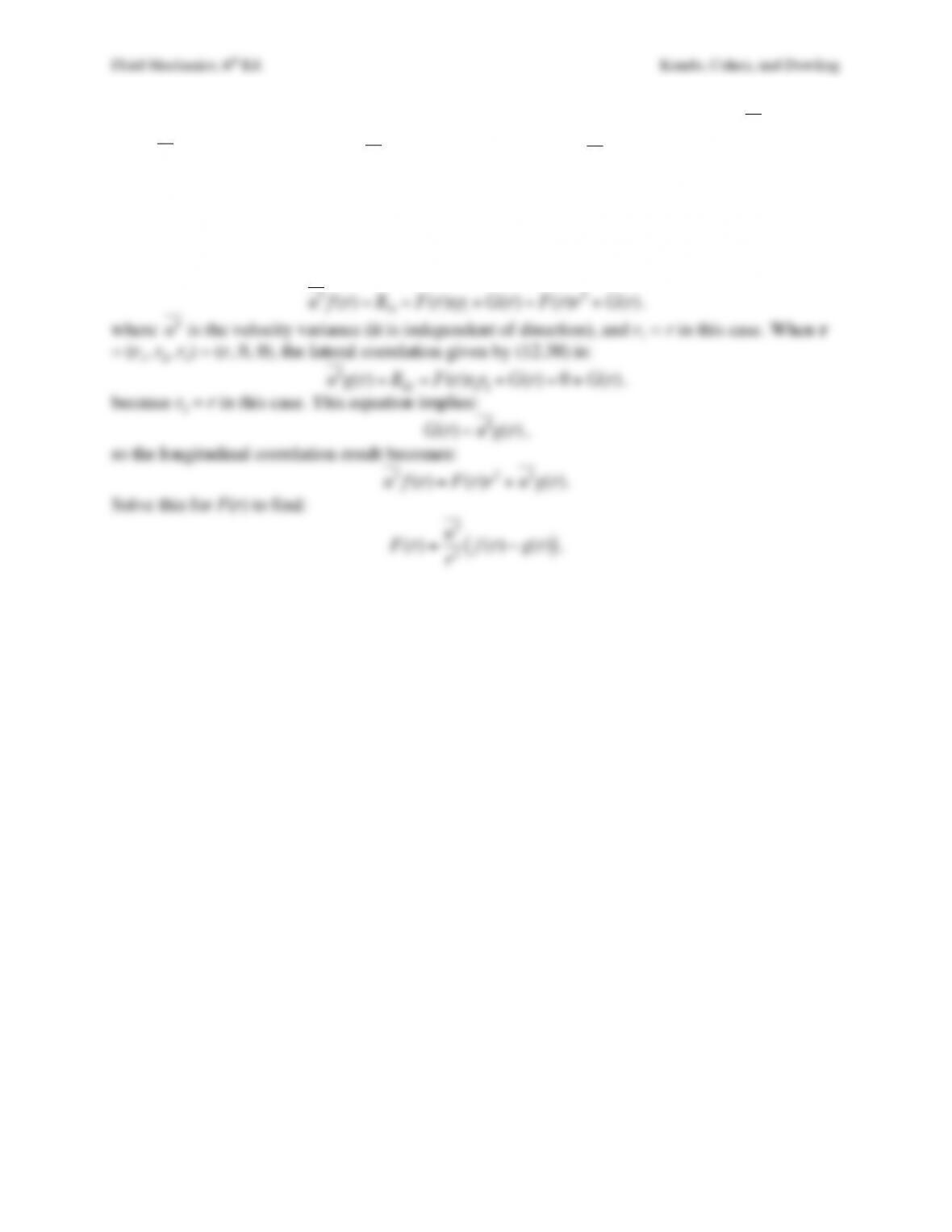
When r = (r1, r2, r3) = (r, 0, 0), the longitudinal correlation given by (12.38) is:
u2f(r)=R11 =F(r)r
1r
1+G(r)=F(r)r2+G(r)
.
where
u2
is the velocity variance (it is independent of direction), and r1 = r in this case. When r
= (r1, r2, r3) = (r, 0, 0), the lateral correlation given by (12.38) is:
u2g(r)=R22 =F(r)r2r2+G(r)=0+G(r)
.
because r2 = r in this case. This equation implies:
G(r)=u2g(r)
,
so the longitudinal correlation result becomes:
u2f(r)=F(r)r2+u2g(r)
.
Solve this for F(r) to find:
F(r)=u2
r2f(r)−g(r)
( )
.
Fluid Mechanics, 6th Ed. Kundu, Cohen, and Dowling
Exercise 12.19. a) Starting from Rij from (12.39), compute
∂
Rij
∂
rj
for incompressible flow.
b) For homogeneous-isotropic turbulence use the result of part a) to show that the longitudinal,
f(r)
, and transverse,
g(r)
, correlation functions are related by
g(r)=f(r)+r2
( )
df (r)dr
( )
.
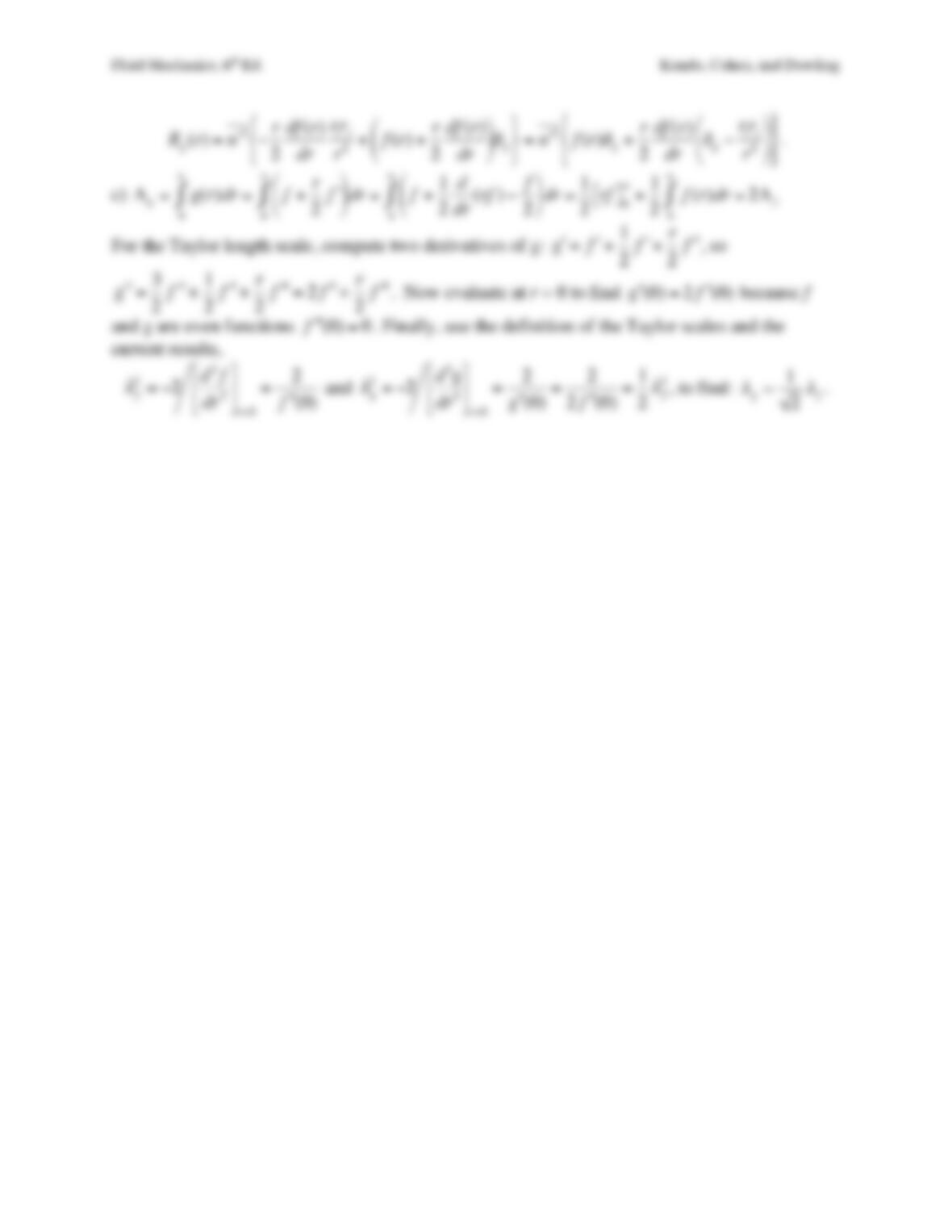
c) Use part b), and the integral length scale and Taylor microscale definitions to find
2Λg=Λf
and
2
λ
g=
λ
f
.
Solution 12.19. a)
∂
∂
rj
Rij =ui(x)
∂
∂
rj
uj(x+r)=0
because the fluctuating velocity field is
incompressible.
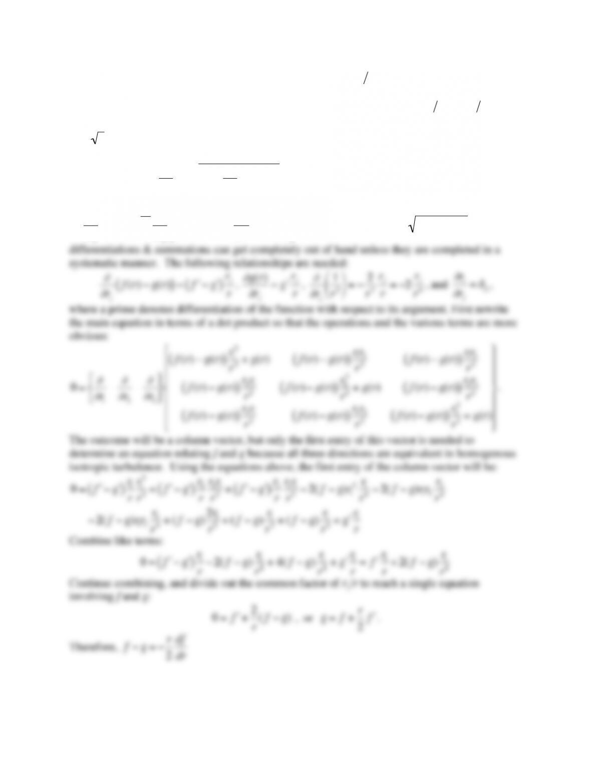
b)
∂
∂
rj
Rij =0=u2
∂
∂
rj
f(r)−g(r)
( )
rirj
r2+g(r)
δ
ij
%
&
'
(
)
*
. At this point with
r=r
1
2+r
2
2+r
3
2
, so the
differentiations & summations can get completely out of hand unless they are completed in a
Fluid Mechanics, 6th Ed. Kundu, Cohen, and Dowling
Fluid Mechanics, 6th Ed. Kundu, Cohen, and Dowling
Exercise 12.20. In homogeneous turbulence:
Rij (rb−ra)=ui(x+ra)uj(x+rb)=Rij (r)
, where
r=rb−ra
.
a) Show that
∂
ui(x)
∂
xk
( )
∂
uj(x)
∂
xl
( )
=−
∂
2Rij
∂
rk
∂
rl
( )
r=0
.
b) If the flow is incompressible and isotropic, show that
−
∂
u1(x)
∂
x1
( )
2=−1
2
∂
u1(x)
∂
x2
( )
2= +2
∂
u1(x)
∂
x2
( )
∂
u2(x)
∂
x1
( )
=u2d2f dr2
( )
r=0
[Hint: expand f(r) about r = 0 before taking any derivatives.]
Solution 12.20. a) Start with
Rij (rb−ra)=ui(x+ra)uj(x+rb)
and take the divergence with
respect to the r-variables.
∂
∂
rb,k
Rij (rb−ra)=
∂
∂
rk
Rij (r)=ui(x+ra)
∂
∂
rb,k
uj(x+rb)=ui(x+ra)
∂
∂
xk
uj(x+rb)
∂
2
∂
ra,l
∂
rb,k
Rij (rb−ra)=−
∂
2
∂
rl
∂
rk
Rij (r)=
∂
∂
ra,l
ui(x+ra)
∂
∂
rb,k
uj(x+rb)=
∂
∂
xl
ui(x+ra)
∂
∂
xk
uj(x+rb)
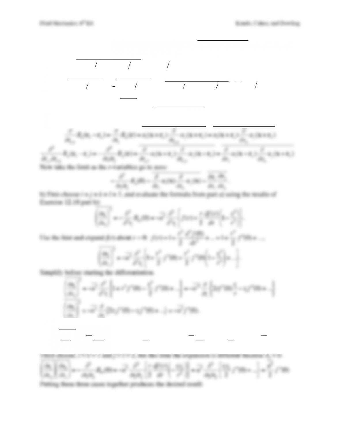
Now take the limit as the r-variables go to zero:
−
∂
2
∂
rl
∂
rk
Rij (0) =
∂
∂
xl
ui(x)
∂
∂
xk
uj(x)=
∂
ui
∂
xl
∂
uj
∂
xk
.
b) First choose i = j = k = l = 1, and evaluate the formula from part a) using the results of
Exercise 12.18 part b):
∂
u1
∂
x1
#
$
%
&
'
(
2
=−
∂
2
∂
2r
1
R11(0) =−u2
∂
2
∂
2r
1
f(r)+r
2
df (r)
dr 1−r
1
2
r2
#
$
%
&
'
(
*
+
,
-
.
/
.
Use the hint and expand f(r) about r = 0:
f(r)=1+r2
2
d2f(0)
dr2+... =1+r2
2" "
f (0) +...
,
∂
u1
∂
x1
#
$
%
&
'
(
2
=−u2
∂
2
∂
2r
1
1+r2
2* *
f (0) +r2
2* *
f (0) 1−r
1
2
r2
#
$
%
&
'
( +...
+
,
-
.
/
0
.
Simplify before starting the differentiation.
∂
u1
∂
x1
#
$
%
&
'
(
2
=−u2
∂
2
∂
2r
1
1+r2* *
f (0) −r
1
2
2* *
f (0) +...
+
,
-
.
/
0 =−*
u 2
∂
∂
r
1
2r* *
f (0) r
1
r−r
1* *
f (0) +...
+
,
-
.
/
0
∂
u1
∂
x1
#
$
% &
'
(
2
=−u2
∂
∂
r
1
2r
1* *
f (0) −r
1* *
f (0) +...
{ }
=−u2* *
f (0)
.
Second choose i = j = 1 and k = l = 2, and use the same expansion
∂
u1
∂
x2
#
$
%
&
'
(
2
=−u2
∂
2
∂
2r2
1+r2* *
f (0) −r
1
2
2* *
f (0) +...
+
,
-
.
/
0 =−u2
∂
∂
r2
2r* *
f (0) r2
r+...
+
,
-
.
/
0 =−2u2* *
f (0)
Third choose, i = k = 1 and j = l = 2, but this time the expansion is different because
δ
ij = 0.
Fluid Mechanics, 6th Ed. Kundu, Cohen, and Dowling
Fluid Mechanics, 6th Ed. Kundu, Cohen, and Dowling
Exercise 12.21. The turbulent kinetic energy equation contains a pressure-velocity correlation,
Kj=p(x)uj(x+r)
. In homogeneous isotropic turbulent flow, the most general form of this
correlation is:
Kj=K(r)rj
. If the flow is also incompressible, show that K(r) must be zero.
Solution 12.21. Compute the divergence of Kj:
∂
∂
rj
Kj=p(x)
∂
∂
rj
uj(x+r)=0
.
because the flow is incompressible. Now insert the homogeneous-isotropic form of Kj.
Fluid Mechanics, 6th Ed. Kundu, Cohen, and Dowling
Exercise 12.22. The velocity potential for two-dimensional water waves of small amplitude
ξ
o
on a deep pool can be written:
φ
(x1,x2,t)=
ωξ
o
k
e+kx2cos
ω
t−kx1
( )
where x1 and x2 are the horizontal and vertical coordinates with x2 = 0 defining the average free
surface. Here,
ω
is the temporal radian frequency of the waves and k is the wave number.
a) Compute the two-dimensional velocity field:
u=(u1,u2)=
∂φ ∂
x1,
∂φ ∂
x2
( )
.
b) Show that this velocity field is a solution of the two-dimensional continuity and Navier-Stokes
equations for incompressible fluid flow.
c) Compute the strain rate tensor
Sij =1
2
∂
ui
∂
xj+
∂
uj
∂
xi
( )
.
d) Although this flow is not turbulent, it must still satisfy the turbulent kinetic energy equation
that contains an energy dissipation term. Denote the kinematic viscosity by
ν
, and compute the
kinetic energy dissipation rate in this flow:
ε
=2
ν
Sij Sij
where the over bar implies a time average
over one wave period = 2
π
/
ω
. Only time averages of even powers of the trig-functions are non-
zero, for example:
cos2
ω
t−kx
( )
=sin2
ω
t−kx
( )
=1 2
while
cos
ω
t−kx
( )
=sin
ω
t−kx
( )
=0
.
e) The original potential represents a lossless flow and does not include any viscous effects.
Explain how this situation can occur when the kinetic-energy dissipation rate is not zero.
Solution 12.22. a) Using the prescribed potential
φ
(x1,x2,t)=
ωξ
o
k
e+kx2cos
ω
t−kx1
( )
, the velocity
field is obtained by differentiation:
ui=
∂φ
∂
x1
,
∂φ
∂
x2
$
%
&
'
(
) =
ωξ
oe+kx2sin
ω
t−kx1
( )
,cos
ω
t−kx1
( )
( )
.
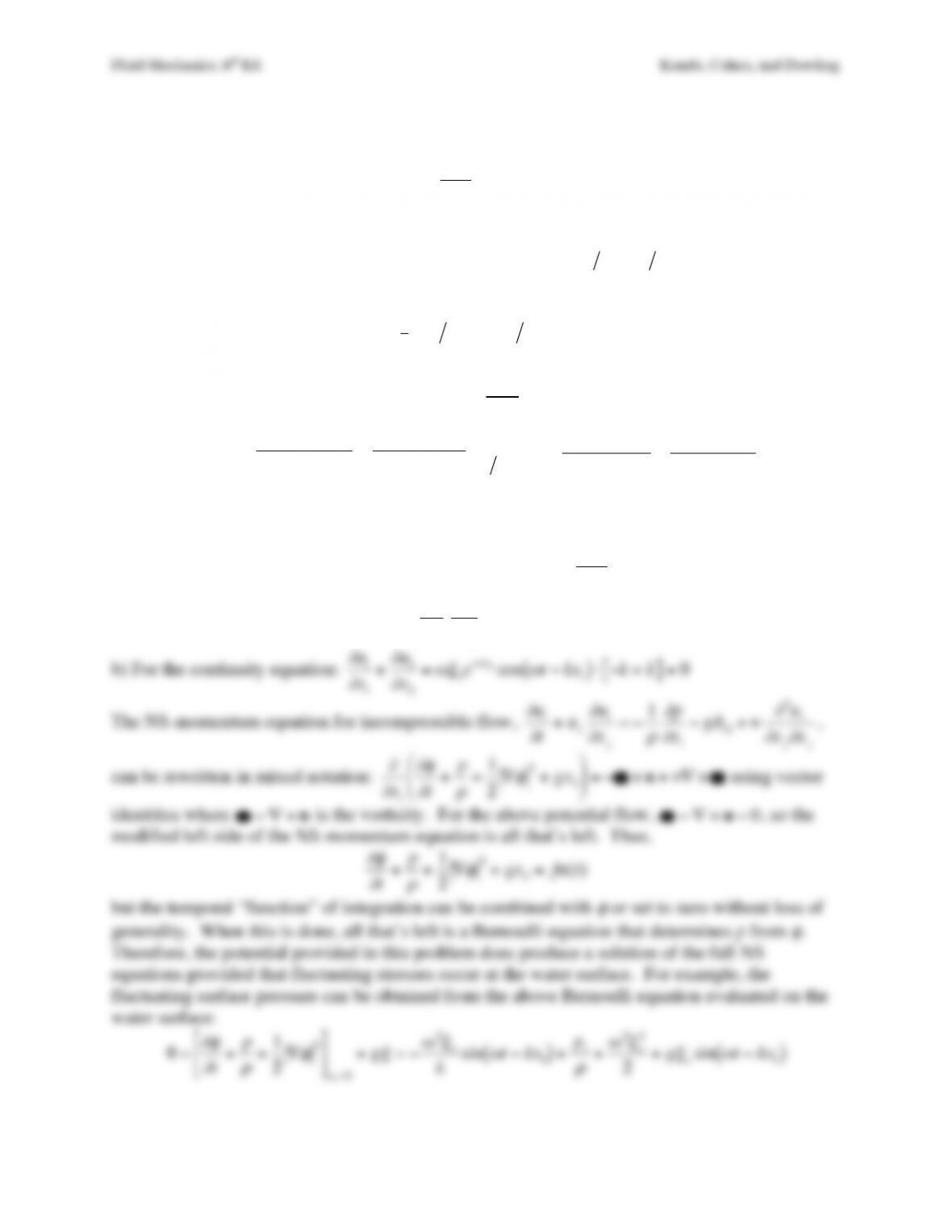
b) For the continuity equation:
∂
u
1
∂
x1
+
∂
u2
∂
x2
=
ωξ
oe+kx2cos
ω
t−kx1
( )
⋅ −k+k
[ ]
=0
Fluid Mechanics, 6th Ed. Kundu, Cohen, and Dowling
where ps is the surface pressure. The usual dispersion relationship for deep water waves,
ω
2=gk
, allows the first and final terms to cancel, leaving
ps
ρ
=−
ω
2
ξ
o
2
2
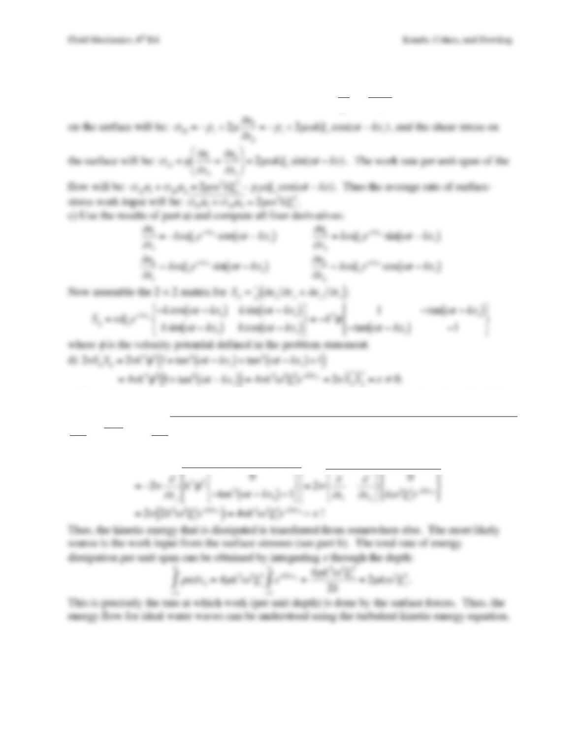
. Thus, the normal stress
on the surface will be:
σ
22 =−ps+2
µ∂
u2
∂
x2
=−ps+2
µω
k
ξ
ocos(
ω
t−kx1)
, and the shear stress on
e) The turbulent kinetic energy equation contains an energy transfer term on the other side of the
equation that includes the viscosity:
∂
∂
xj
2
ν
uiSij
( )
=2
ν∂
∂
xj
−k2
φωξ
oe+kx2sin
ω
t−kx1
( )
cos
ω
t−kx1
( )
{ }
1−tan
ω
t−kx1
( )
−tan
ω
t−kx1
( )
−1
(
)
*
+
,
-
.
/
0
0
1
2
3
3
=−2
ν∂
∂
xj
k3
φ
20
−tan2
ω
t−kx1
−1
'
(
*
+
-
/
0
2 =2
ν∂
∂
x1
∂
∂
x2
'
(
*
+
0
k
ω
2
ξ
2e+2kx2
'
(
*
+
Fluid Mechanics, 6th Ed. Kundu, Cohen, and Dowling
Exercise 12.23. A mass of 10 kg of water is stirred by a mixer. After one hour of stirring, the
temperature of the water rises by 1.0 °C. What is the power output of the mixer in watts? What is
the size
η
of the dissipating eddies?
Solution 12.23. Start from a thermodynamic description of the power delivered to the water.
Power =
mCpΔT
Δt=(10kg)(4200m2s−2K−1)(1K)
3600s=11.67W
The kinetic energy dissipation rate per unit mass is:
Fluid Mechanics, 6th Ed. Kundu, Cohen, and Dowling
Exercise 12.24. In locally isotropic turbulence, A.N. Kolmogorov determined that the wave
number spectrum can be represented by
S11(k)
ν
5
ε
( )
1 4 =Φk
ν
3 4
ε
1 4
( )
in the inertial-subrange
and dissipation-range of turbulent scales, where Φ is an undetermined function.
a) Determine the equivalent form for the temporal spectrum
Se(
ω
)
in term of the average kinetic
energy dissipation rate
ε
, the fluid’s kinematic viscosity
ν
, and the temporal frequency
ω
.
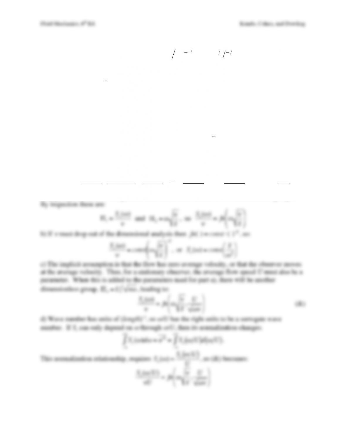
b) Simplify the results of part a) for the inertial range of scales where
ν
is dropped from the
dimensional analysis.
c) To obtain the results for parts a) and b) an implicit assumption has been made that leads to the
neglect of an important parameter. Add the missing parameter and redo the dimensional analysis
of part a).
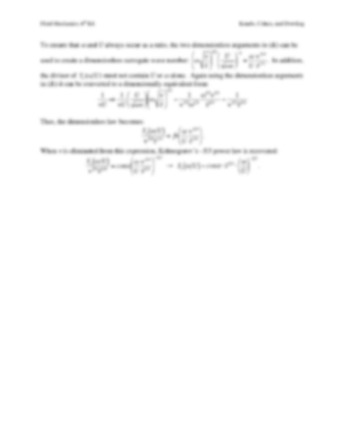
d) Use the missing parameter and
ω
to develop an equivalent wave number. Insist that your
result for Se only depend on this equivalent wave number and
ε
to recover the minus-five-thirds
law.
Solution 12.24. a) First layout the units of the various quantities using square brackets to denote
“units of”.
Se(
ω
)
[ ]
=length2
time2⋅1
frequency =length2
time
,
ε
[ ]
=length2
time3
,
ν
[ ]
=length2
time
, and
ω
[ ]
=1
time
.
Four parameters and two independent units means there should be two dimensionless groups.
By inspection these are:
Fluid Mechanics, 6th Ed. Kundu, Cohen, and Dowling
Fluid Mechanics, 6th Ed. Kundu, Cohen, and Dowling
Exercise 12.25. Estimates for the importance of anisotropy in a turbulent flow can be developed
by assuming that fluid velocities and spatial derivatives of the average-flow (or RANS) equation
are scaled by the average velocity difference ΔU that drives the largest eddies in the flow having
a size L, and that the fluctuating velocities and spatial derivatives in the turbulent kinetic energy
(TKE) equation are scaled by the kinematic viscosity
ν
and the Kolmogorov scales
η
and uK [see
(12.50)]. Thus, the scaling for a mean velocity gradient is:
∂
Ui
∂
xj~ΔU L
, while the mean-
square turbulent velocity gradient scales as:
∂
ui
∂
xj
( )
2
~uK
η
( )
2=
ν
2
η
4
, where the “~” sign
means “scales as”. Use these scaling ideas in parts a) and d) below.
a) The total energy dissipation rate in a turbulent flow is
2
ν
S
ij S
ij +2
ν
#
S
ij #
S
ij
, where
S
ij =1
2
∂
Ui
∂
xj
+
∂
Uj
∂
xi
#
$
%
%
&
'
(
(
and
"
S
ij =1
2
∂
ui
∂
xj
+
∂
uj
∂
xi
$
%
&
&
'
(
)
)
. Determine how the ratio
"
S
ij "
S
ij
S
ij S
ij
depends on the
outer-scale Reynolds number:
ReL=ΔU⋅L
ν
.
b) Is average-flow or fluctuating-flow energy dissipation more important?
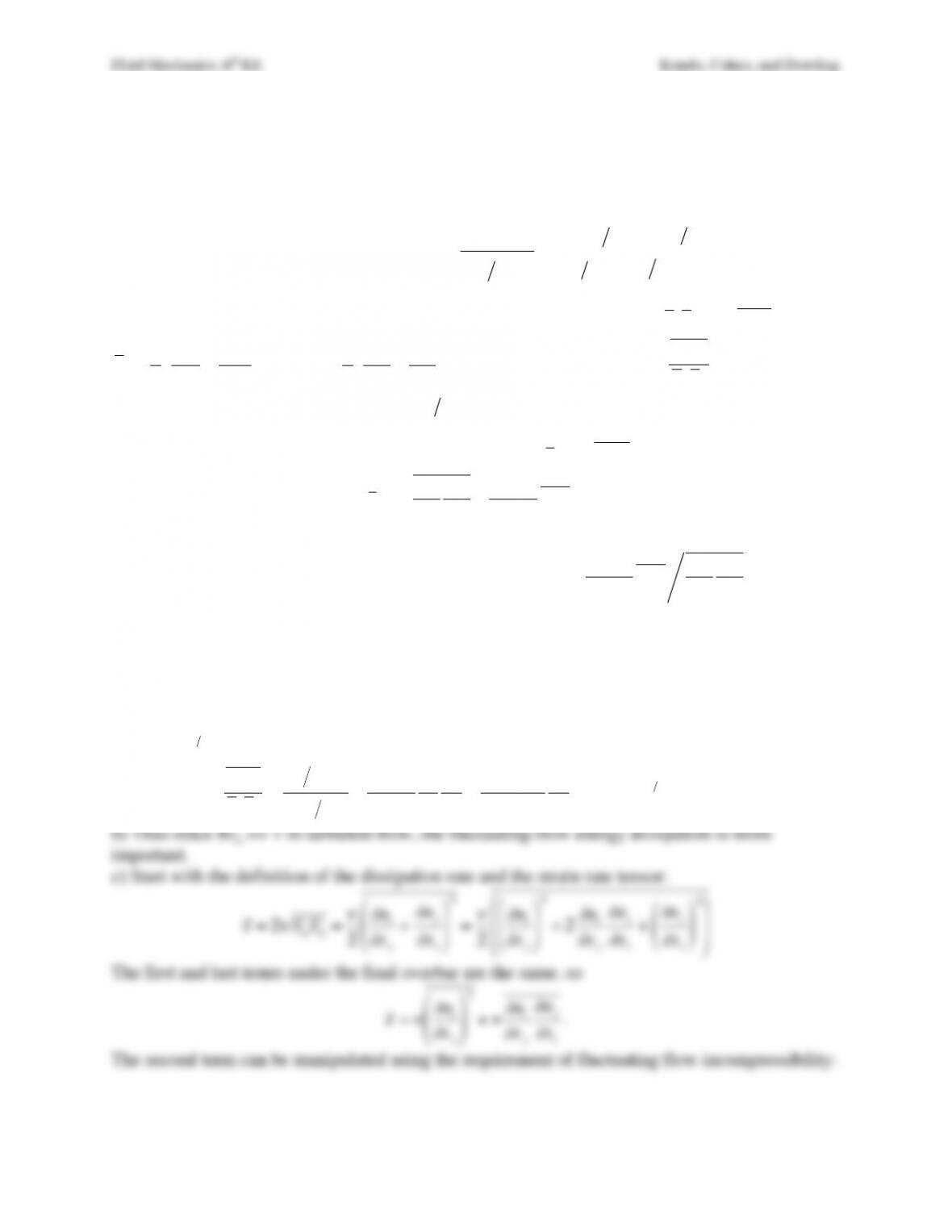
c) Show that the turbulent kinetic energy dissipation rate,
ε
=2
ν
$
S
ij $
S
ij
can be written:
ε
=
ν∂
ui
∂
xj
∂
ui
∂
xj
+
∂
2
∂
xi
∂
xj
uiuj
%
&
'
(
)
*
.
d) For homogeneous isotropic turbulence, the second term in the result of part c) is zero but it is
non-zero in a turbulent shear flow. Therefore, estimate how
∂
2
∂
xi
∂
xj
uiuj
∂
ui
∂
xj
∂
ui
∂
xj
depends on
ReL in turbulent shear flow as means of assessing how much impact anisotropy has on the
turbulent kinetic energy dissipation rate.
e) Is an isotropic model for the turbulent dissipation appropriate at high ReL in a turbulent shear
flow?
Solution 12.25. a) Use the scaling ideas in the problem statement and the relationship
η
∝L⋅Re−3 4
to find:
"
S
ij "
S
ij
S
ij S
ij
~
ν η
2
( )
2
ΔU L
( )
2=
ν
2L2
(ΔU)2
L4
L4
1
η
4=
ν
2
(ΔU)2L2
L4
η
4=ReL
−2ReL
3 4
( )
4=ReL
b) Thus since ReL >> 1 in turbulent flow, the fluctuating-flow energy dissipation is more
Fluid Mechanics, 6th Ed. Kundu, Cohen, and Dowling
Fluid Mechanics, 6th Ed. Kundu, Cohen, and Dowling
Exercise 12.26. Determine the self-preserving form of the average stream-wise velocity Uz(z,R)
of a round turbulent jet using cylindrical coordinates where z increases along the jet axis and R is
the radial coordinate. Ignore gravity in your work. Denote the density of the nominally-quiescent
reservoir fluid by
ρ
.
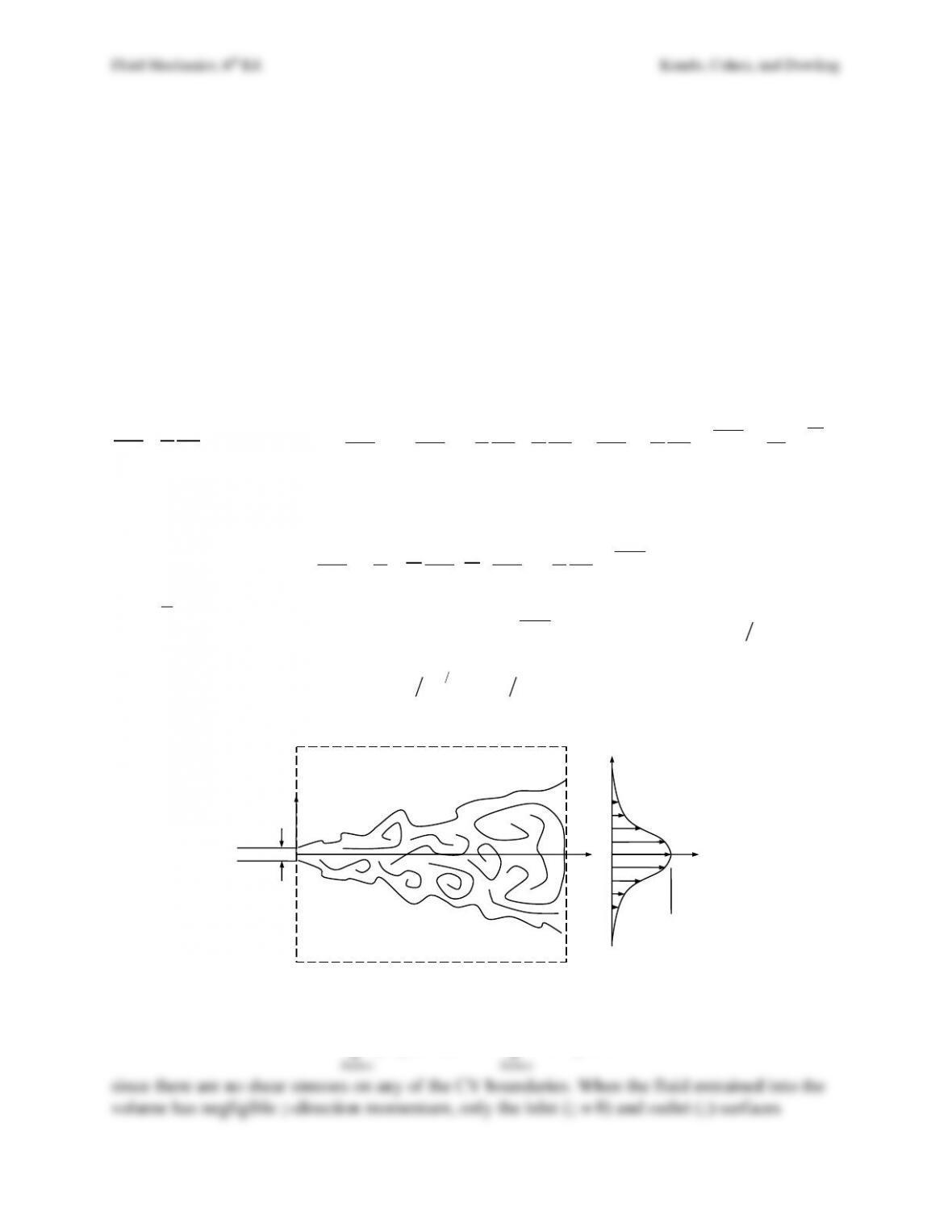
a) Place a stationary cylindrical control volume around the jet's cone of turbulence so that
circular control surfaces slice all the way through the jet flow at its origin and at a distance z
downstream where the fluid density is
ρ
. Assuming that the fluid outside the jet is nearly
stationary so that pressure does not vary in the axial direction and that the fluid entrained into the
volume has negligible x-direction momentum, show
J0≡
ρ
0U0
2
0
d/2
∫2
π
RdR =
ρ
Uz
2(z,R)2
π
0
D/2
∫RdR
,
where J0 is the jet's momentum flux,
ρ
0 is the density of the jet fluid, and U0 is the jet exit
velocity.
b) Simplify the exact mean-flow equations
∂
Uz
∂
z+1
R
∂
∂
R
RUR
( )
=0
, and
Uz
∂
Uz
∂
z+UR
∂
Uz
∂
R=−1
ρ
∂
P
∂
z+
ν
R
∂
∂
R
R
∂
Uz
∂
R
"
#
$%
&
'−1
R
∂
∂
R
RuzuR
( )
−
∂
∂
z
Ruz
2
()
,
when ∂P/∂z ≈ 0, the jet is slender enough for the boundary layer approximation ∂/∂R >> ∂/∂z to
be valid, and the flow is at high Reynolds number so that the viscous terms are negligible.
c) Eliminate the average radial velocity from the simplified equations to find:
Uz
∂
Uz
∂
z−1
R
R
∂
Uz
∂
z
dR
0
R
∫
#
$
%
&
'
(
∂
Uz
∂
R=−1
R
∂
∂
R
RuzuR
( )
where R is just an integration variable.
d) Assume a similarity form:
Uz(z,R)=UCL (z)f(
ξ
)
,
−uzuR=Ψ(z)g(
ξ
)
, where
ξ
=R
δ
(z)
and f
and g are undetermined functions, use the results of parts a) and c), and choose constant values
appropriately to find
Uz(z,R)=const.J0
ρ
( )
1 2 z−1f R z
( )
.
e) Determine a formula for the volume flux in the jet. Will the jet fluid from the nozzle be diluted
with increasing z?
Solution 12.26. a) Use the stationary CV shown above, consider only the steady mean flow, and
ignore turbulent fluctuations. In this case the CV momentum equation is:
ρ
Uz(U⋅n)
Surface
∫dA =−Pn⋅ezdA
Surface
∫
,
since there are no shear stresses on any of the CV boundaries. When the fluid entrained into the
z!
R!
Uz(z,R)!
UCL(z)!
d!
Fluid Mechanics, 6th Ed. Kundu, Cohen, and Dowling
Fluid Mechanics, 6th Ed. Kundu, Cohen, and Dowling
Now reassemble (3*) and cancel terms.
UCL "
U
CL f2−UCL
2f"
f
ξ
"
δ
δ
−UCL "
U
CL "
f
ξ
+2UCL
2"
f
ξ
"
δ
δ
&
'
(
)
*
+ f
ξ
d
ξ
0
ξ
∫+UCL
2
ξ
f"
f "
δ
δ
=RSCL
δξ
∂
∂ξ ξ
g
( )
UCL "
U
CL f2−UCL "
U
CL "
f
ξ
+2UCL
2"
f
ξ
"
δ
δ
&
'
(
)
*
+ f
ξ
d
ξ
0
ξ
∫=RSCL
δξ
∂
∂ξ ξ
g
( )
Multiply by
δ
and divide by
UCL
2
to find:


