Fluid Mechanics, 6th Ed. Kundu, Cohen, and Dowling
Exercise 12.1. Determine general relationships for the second, third, and four central moments
(variance =
σ
2, skewness = S, and kurtosis = K) of the random variable u in terms of its first four
ordinary moments:
u
,
u2
,
u3
, and
u4
.
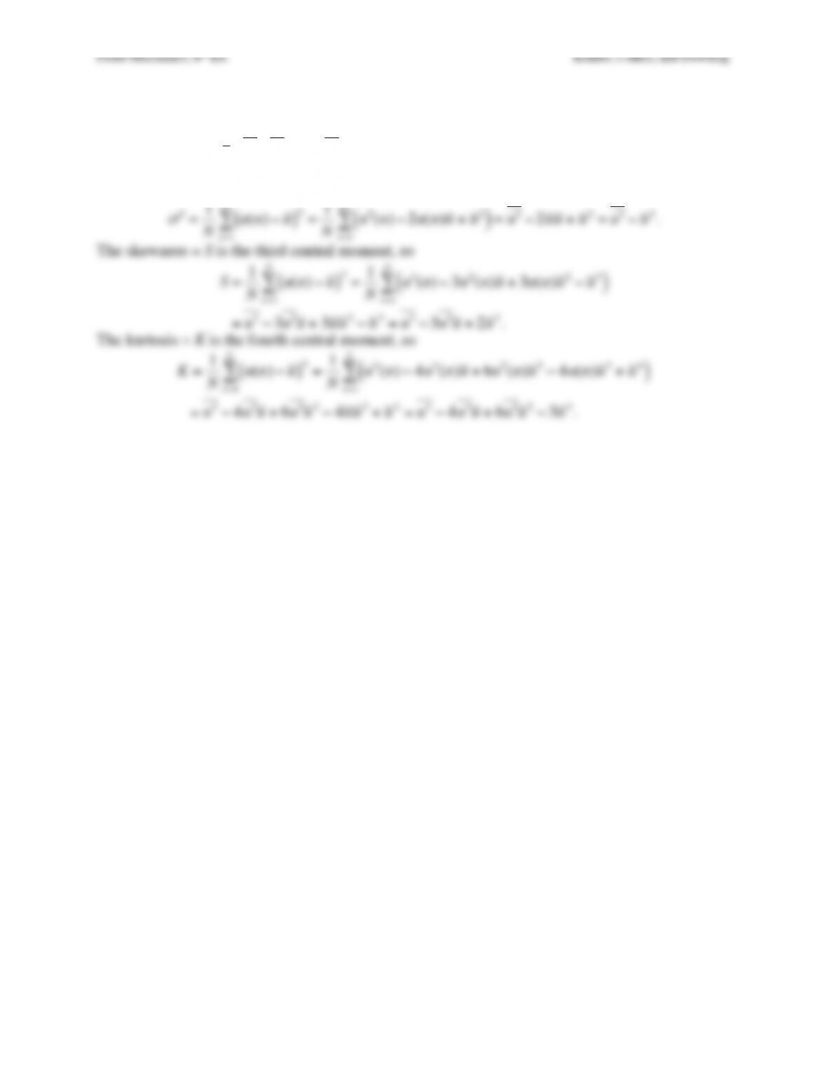
Solution 12.1. a) The variance =
σ
2 is the second central moment, so:
σ
2=1
N
u(n)−u
( )
2
n=1
N
∑=1
N
u2(n)−2u(n)u +u
2
( )
n=1
N
∑=u2−2u u +u
2=u2−u
2
.
The skewness = S is the third central moment, so
S=1
N
u(n)−u
( )
3
n=1
N
∑=1
N
u3(n)−3u2(n)u +3u(n)u
2−u
3
( )
n=1
N
∑
=u3−3u2u +3u u
2−u
3=u3−3u2u +2u
3.
The kurtosis = K is the fourth central moment, so
K=1
N
u(n)−u
( )
4
n=1
N
∑=1
N
u4(n)−4u3(n)u +6u2(n)u
2−4u(n)u
3+u
4
( )
n=1
N
∑
=u4−4u3u +6u2u
2−4u u
3+u
4=u4−4u3u +6u2u
2−3u
4.
Fluid Mechanics, 6th Ed. Kundu, Cohen, and Dowling
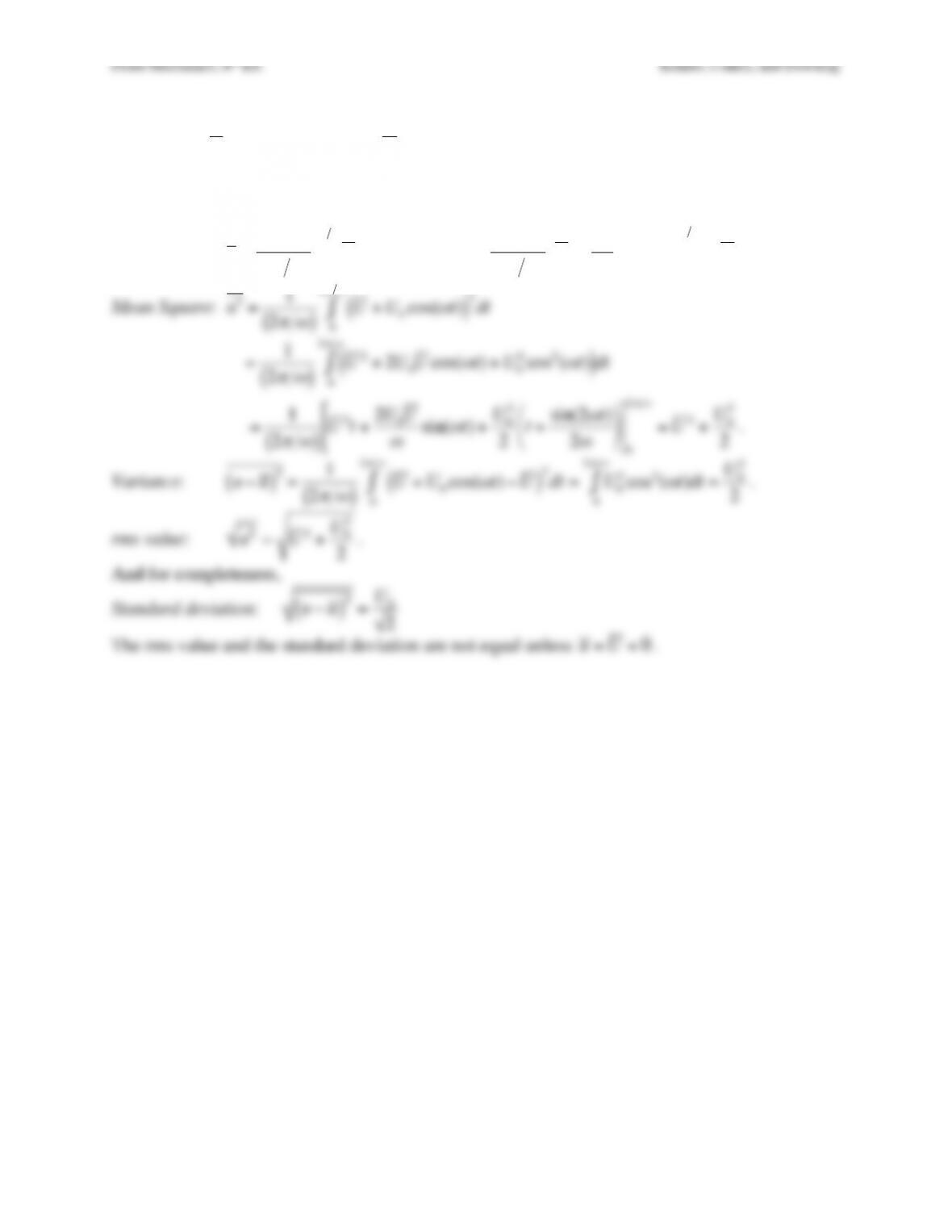
Exercise 12.2. Calculate the mean, mean square, variance, and rms value of the periodic time
series
u(t)=U +U0cos
ω
t
( )
, where
U
, U0 and
ω
are positive real constants.
Solution 12.2. The given time series is periodic so time averaging over one period will yield the
desired results.
Average:
u =1
2
π ω
( )
U +U0cos(
ω
t)
( )
0
2
π ω
∫dt =1
2
π ω
( )
U t+U0
ω
sin(
ω
t)
%
&
‘
(
)
*
0
2
π ω
=U
.
Mean Square:
u2=1
2
π ω
U +U0cos(
ω
t)
( )
2
2
π ω
∫dt
Fluid Mechanics, 6th Ed. Kundu, Cohen, and Dowling
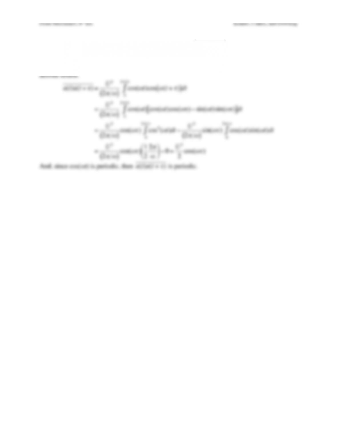
Exercise 12.3. Show that the autocorrelation function
u(t)u(t+
τ
)
of a periodic series u =
Ucos(
ω
t) is itself periodic.
Solution 12.3. The given time series is periodic so time averaging over one period will yield the
desired results.
u(t)u(t+
τ
)
Fluid Mechanics, 6th Ed. Kundu, Cohen, and Dowling
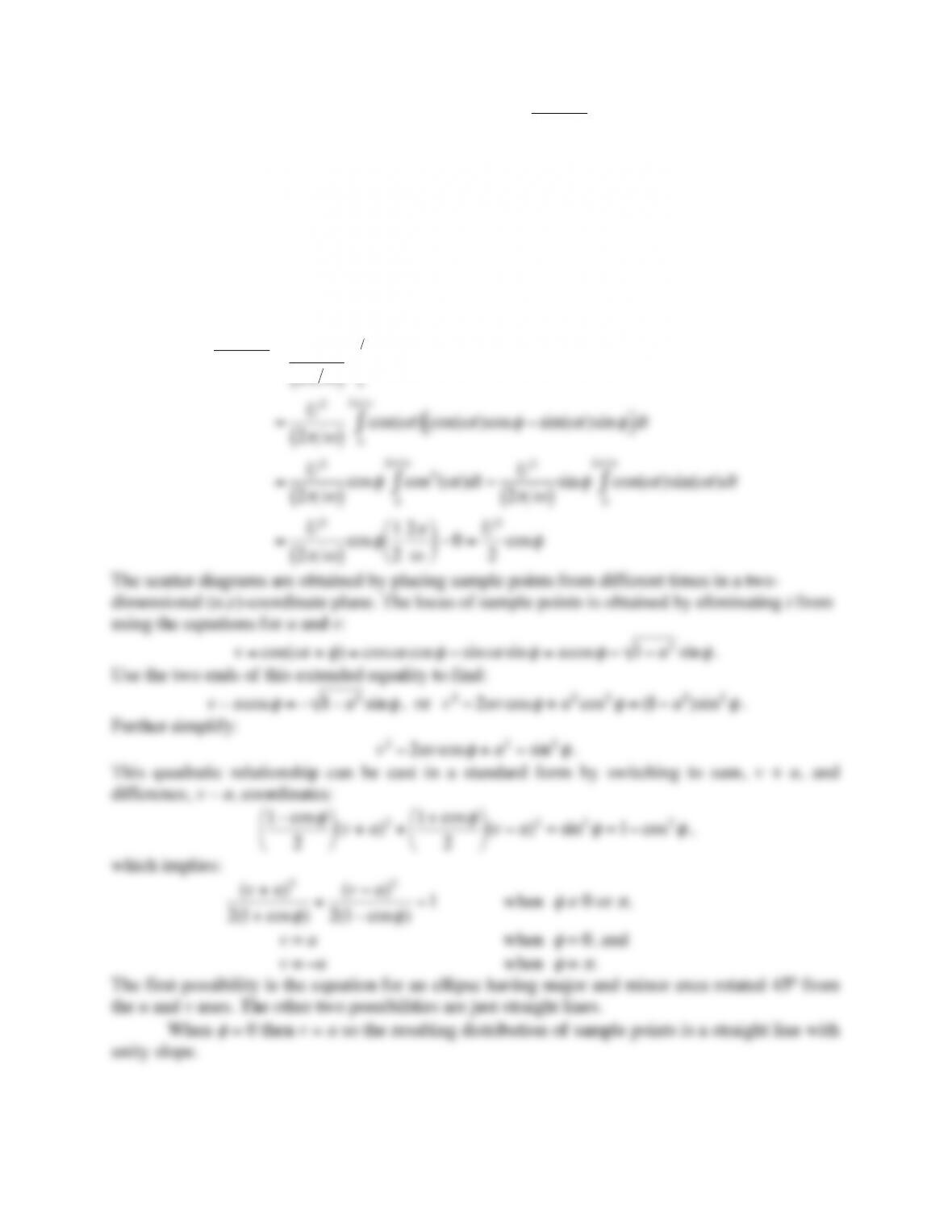
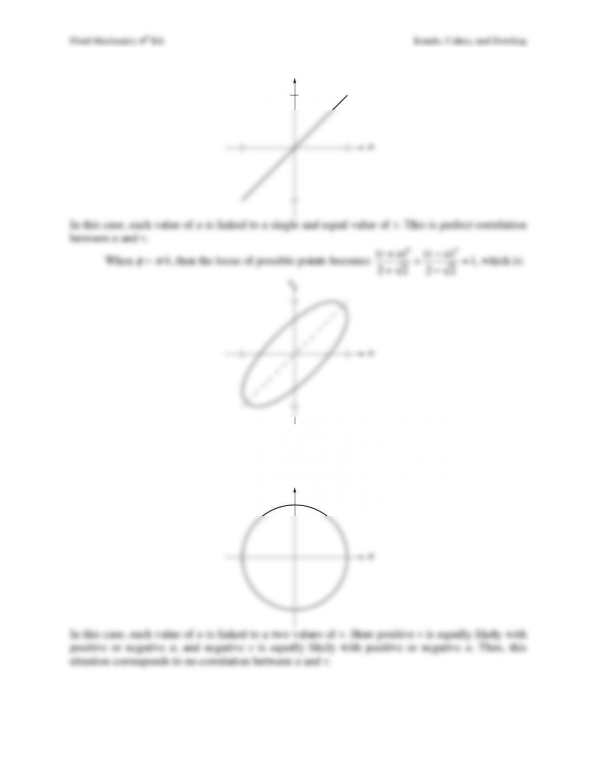
Exercise 12.4. Calculate the zero-lag cross-correlation
u(t)v(t)
between two periodic series u(t)
= cos
ω
t and v(t) = cos(
ω
t +
φ
) by performing at time average over one period = 2π/
ω
. For values
of
φ
= 0,
π
/4, and
π
/2, plot the scatter diagrams of u vs v at different times, as in Figure 12.8.
Note that the plot is a straight line if
φ
= 0, an ellipse if
φ
=
π
/4, and a circle if
φ
=
π
/2; the
straight line, as well as the axes of the ellipse, are inclined at 45° to the uv-axes. Argue that the
straight line signifies a perfect correlation, the ellipse a partial correlation, and the circle a zero
correlation.
Solution 12.4. The given time series is periodic so time averaging over one period will yield the
desired results.
u(t)v(t)=U2
2
π ω
( )
cos(
ω
t)cos
ω
t+
φ
( )
0
2
π ω
∫dt
=U2
2
π ω
( )
cos(
ω
t) cos(
ω
t)cos
φ
−sin(
ω
t)sin
φ
[ ]
0
2
π ω
∫dt
=U2
2
π ω
( )
cos
φ
cos2(
ω
t)
0
2
π ω
∫dt −U2
2
π ω
( )
sin
φ
cos(
ω
t)
0
2
π ω
∫sin(
ω
t)dt
=U2
2
π ω
( )
cos
φ
1
2
2
π
ω
‘
(
) *
+
, −0=U2
2cos
φ
The scatter diagrams are obtained by placing sample points from different times in a two-
dimensional (u,v)-coordinate plane. The locus of sample points is obtained by eliminating t from
using the equations for u and v:
v=cos(
ω
t+
φ
)=cos
ω
tcos
φ
−sin
ω
tsin
φ
=ucos
φ
−1−u2sin
φ
.
Use the two ends of this extended equality to find:
v−ucos
φ
=−1−u2sin
φ
, or
v2−2uv cos
φ
+u2cos2
φ
=(1−u2)sin2
φ
.
Further simplify:
v2−2uv cos
φ
+u2=sin2
φ
.
This quadratic relationship can be cast in a standard form by switching to sum, v + u, and
difference, v – u, coordinates:
1−cos
φ
2
$
%
& ‘
(
)
(v+u)2+1+cos
φ
2
$
%
& ‘
(
)
(v−u)2=sin2
φ
=1−cos2
φ
,
which implies:
(v+u)2
2(1+cos
φ
)+(v−u)2
2(1−cos
φ
)=1
when
φ
≠ 0 or
π
,
v = u when
φ
= 0, and
v = –u when
φ
=
π
.
The first possibility is the equation for an ellipse having major and minor axes rotated 45° from
the u and v axes. The other two possibilities are just straight lines.
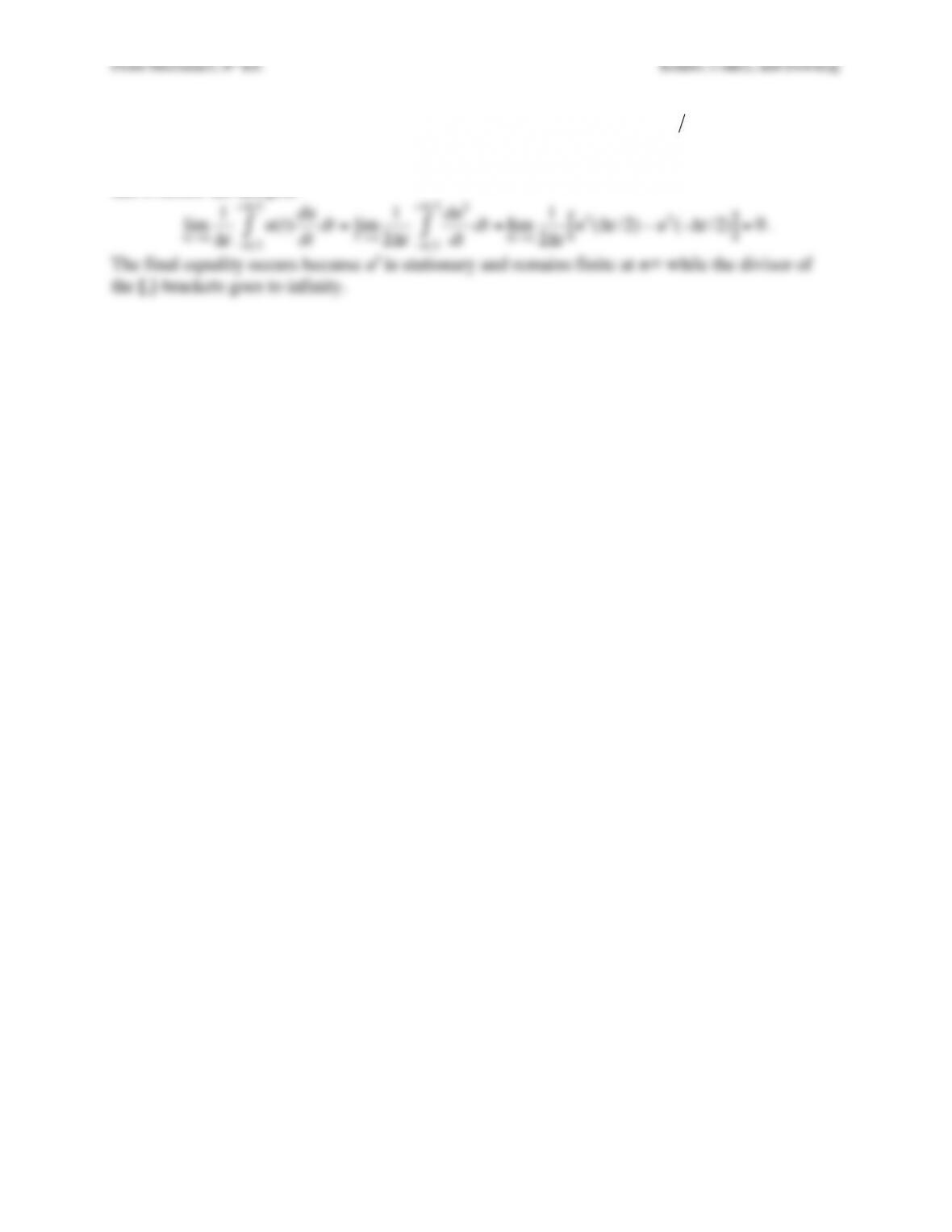
When
φ
= 0 then v = u so the resulting distribution of sample points is a straight line with
unity slope.
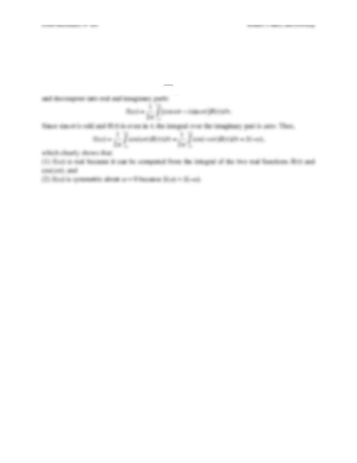
Fluid Mechanics, 6th Ed. Kundu, Cohen, and Dowling
In this case, each value of u is linked to a two values of v. Here positive v is more likely with
positive u, and negative v is more likely with negative u. Thus, this situation corresponds to
partial correlation between u and v.
When
φ
=
π
/2, then the locus of possible points becomes, which is a circle:
u
v
u
v
Fluid Mechanics, 6th Ed. Kundu, Cohen, and Dowling
Exercise 12.5. If u(t) is a stationary random signal, show that u(t) and
du(t)dt
are uncorrelated.
Solution 12.5. a) For a stationary signal u(t), use the time-average definition of the correlation
and evaluate the integral:
lim
Δt→∞
1
Δt
u(t)du
dt
dt
−Δt2
+Δt2
∫=lim
T→∞
1
2Δt
du2
dt
dt =
−Δt2
+Δt2
∫lim
Δt→∞
1
2Δt
u2(Δt/2) −u2(−Δt/2)
[ ]
=0
.
The final equality occurs because u2 is stationary and remains finite at ±∞ while the divisor of
the [,]-brackets goes to infinity.
Fluid Mechanics, 6th Ed. Kundu, Cohen, and Dowling
Exercise 12.6. Let R(
τ
) and S(
ω
) be a Fourier transform pair. Show that S(
ω
) is real and
symmetric if R(
τ
) is real and symmetric.
Solution 12.6. Start with:
S(
ω
)=1
2
π
e−i
ωτ
R(
τ
)d
τ
−∞
+∞
∫
,
and decompose into real and imaginary parts:
Fluid Mechanics, 6th Ed. Kundu, Cohen, and Dowling
Exercise 12.7. Compute the power spectrum, integral time scale, and Taylor time scale when
R
11(
τ
)=u1
2exp −
ατ
2
( )
cos(
ω
o
τ
)
, assuming that
α
and
ω
o are real positive constants.
Solution 12.7.
Se(
ω
)=u1
2
2
π
e−
ατ
2cos(
ω
o
τ
)exp −i
ωτ
{ }
−∞
+∞
∫d
τ
=u1
2
4
π
e−
ατ
2ei(
ω
o−
ω
)
τ
+ei(−
ω
o−
ω
)
τ
( )
d
τ
−∞
+∞
∫
The exponents of the two terms in the integrand are:
−
ατ
2−i(
ω
∓
ω
o)
τ
=−
α τ
2+i(
ω
∓
ω
o)
ατ
+(
ω
∓
ω
o)2
4
α
2−(
ω
∓
ω
o)2
4
α
2
&
‘
(
)
*
+
=−
α τ
+i(
ω
∓
ω
o)
2
α
&
‘
( )
*
+
2
−(
ω
∓
ω
o)2
4
α
,
where the top sign belongs with the first term. Let
β
=
α τ
+i(
ω
∓
ω
o)
2
α
&
‘
( )
*
+
be the new integration
variable:
Se(
ω
)=u1
2
4
π α
exp −(
ω
−
ω
o)2
4
α
&
‘
(
)
*
+
e−
β
2d
β
−∞
+∞
∫+u1
2
4
π α
exp −(
ω
+
ω
o)2
4
α
&
‘
(
)
*
+
e−
β
2d
β
−∞
+∞
∫
.
The integral in both terms is
π
, so the energy spectrum is:
Se(
ω
)=u1
2
4
πα
exp −(
ω
−
ω
o)2
4
α
&
‘
(
)
*
+ +exp −(
ω
+
ω
o)2
4
α
&
‘
(
)
*
+
,
–
.
/
0
1
.
The integral time scale can be determined from (12.18) and (12.20) evaluated at
ω
= 0:
Λt=1
#
u 2
R
11(
τ
)d
τ
=
0
∞
∫2
π
2u1
2
Se(0) =
π
u1
2
u1
2
4
πα
2exp −
ω
o
2
4
α
+
,
–
.
/
0 =
π
2
α
exp −
ω
o
2
4
α
+
,
–
.
/
0
.
The Taylor time scale defined in (12.19) involves the second derivative of R11 at
τ
= 0, which is
tedious to determine directly. However the given R11 is relatively easy to expand for
τ
<< 1:
R
11(
τ
)=u1
2exp −
ατ
2
( )
cos(
ω
o
τ
)=u1
21−
ατ
2+…
( )
1−1
2(
ω
o
τ
)2+…
( )
=u1
21−
α
+1
2
ω
o
2
[ ]
τ
2+…
( )
,
and this is much easier to differentiate:
d2R
11(
τ
)
d
τ
2
#
$
%
&
‘
(
τ
=0
=−u1
22
α
+
ω
o
2
[ ]
.
So,
λ
t=−2R
11(0) d2R
11(
τ
)
d
τ
2
%
&
‘
(
)
*
τ
=0
+
,
–
.
/
0
1 2
=−2u1
2
−u1
22
α
+
ω
o
2
[ ]
=
α
+1
2
ω
o
2
[ ]
−1 2
.
Fluid Mechanics, 6th Ed. Kundu, Cohen, and Dowling
Exercise 12.8. There are two formulae for the energy spectrum Se(
ω
) of the stationary zero-mean
signal
u(t)
:
Se(
ω
)=1
2
π
R
11(
τ
)exp −i
ωτ
{ }
−∞
+∞
∫d
τ
and
Se(
ω
)=lim
T→∞
1
2
π
T
u(t)exp −i
ω
t
{ }
−T2
+T2
∫dt
2
.
Prove these two are identical without requiring the existence of the Fourier transform of
u(t)
.
Solution 12.8. Start with the second formula and use t´ and t as the integration variables.
Se(
ω
)=lim
T→∞
1
2
π
T
u(t)exp −i
ω
t
{ }
−T2
+T2
∫dt
2
=lim
T→∞
1
2
π
T
u((
t )u(t)exp −i
ω
((
t −t)
{ }
−T2
+T2
∫d(
t
−T2
+T2
∫dt
.
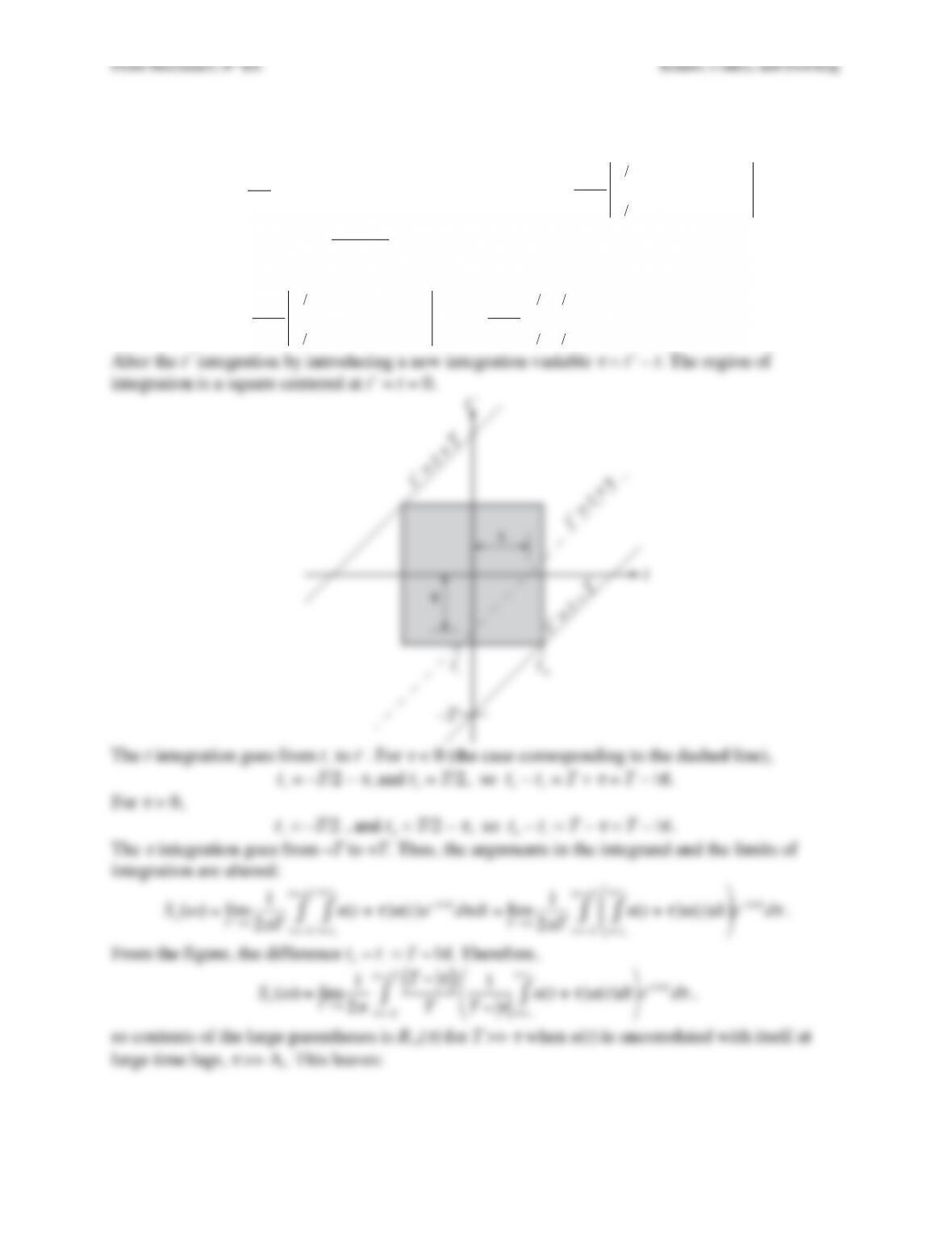
Alter the t´ integration by introducing a new integration variable
τ
= t´ – t. The region of
Se(
ω
)=lim
T→∞
1
2
π
T−
τ
( )
T
1
T−
τ
u(t+
τ
)u(t)
t=t−
∫dt
*
+
–
.
τ
=−T
∫e−i
ωτ
d
τ
,
so contents of the large parentheses is R11(
τ
) for T >>
τ
when u(t) is uncorrelated with itself at
large time lags,
τ
>> Λt. This leaves:
Fluid Mechanics, 6th Ed. Kundu, Cohen, and Dowling
Fluid Mechanics, 6th Ed. Kundu, Cohen, and Dowling
Exercise 12.9. Derive the formula for the temporal Taylor microscale
λ
t by expanding the
definition of the temporal correlation function (12.17) into a two term Taylor series, and
determining the time shift,
τ
=
λ
t, where this two term expansion equals zero.
Solution 12.9. Expand the temporal autocorrelation:
R
11(
τ
)=R
11(0) +
τ
dR
11(
τ
)
d
τ
#
$
% &
‘
(
τ
=0
+
τ
2
2
d2R
11(
τ
)
d
τ
2
#
$
%
&
‘
(
τ
=0
+…
The autocorrelation function is even, so the terms involving odd derivatives are zero. Thus, the
Fluid Mechanics, 6th Ed. Kundu, Cohen, and Dowling
Exercise 12.10. When x, r, and k1 all lie in the stream-wise direction, the wave number spectrum
S11(k1)
of the stream-wise velocity fluctuation
u1(x)
defined by (12.45) can be interpreted as a
distribution function for energy across stream-wise wave number k1. Show that the energy-
weighted mean-square value of the stream-wise wave number is:
k1
2≡1
u2
k1
2S11(k1)dk1=−1
u2
−∞
+∞
∫d2
dr2R
11(r)
&
‘
(
)
*
+
r=0
, and that
λ
f=2k1
2
.
Solution 12.10. The relationship between the stream-wise autocorrelation function and the
stream-wise spatial power spectrum is the Fourier inverse of (12.45):
R
11(r)=S11(k1)e+ik1rdk1
−∞
+∞
∫
.
Differentiate this twice with respect to r, and evaluate at r = 0:
2
Fluid Mechanics, 6th Ed. Kundu, Cohen, and Dowling
Exercise 12.11. In many situations, measurements are only possible of one velocity component
at one point in a turbulent flow, but the flow has a non-zero mean velocity and moves past the
measurement point. Thus, the experimenter obtains a time history of
u1(t)
at fixed point. In
order to estimate spatial velocity gradients, Taylor’s frozen-turbulence hypothesis can be
invoked to estimate a spatial gradient from a time derivative:
∂
u
1
∂
x1
≈ − 1
U1
∂
u
1
∂
t
where the “1”-axis
must be aligned with the direction of the average flow, i.e. Ui = (U1, 0, 0). Show that this
approximate relationship is true when
uiuiU1<< 1
,
p~
ρ
u1
2
, and Re is high enough to neglect
the influence of viscosity.
Solution 12.11. The place to start is with the “1”-component of the Navier-Stokes equation for
an incompressible fluid:
∂
u1
∂
t+u1
∂
u1
∂
x1
+u2
∂
u1
∂
x2
+u3
∂
u1
∂
x3
=−1
ρ
∂
p
∂
x1
+
ν∂
2u1
∂
x1
2+
∂
2u1
∂
x2
2+
∂
2u1
∂
x3
2
&
‘
(
)
*
+
.
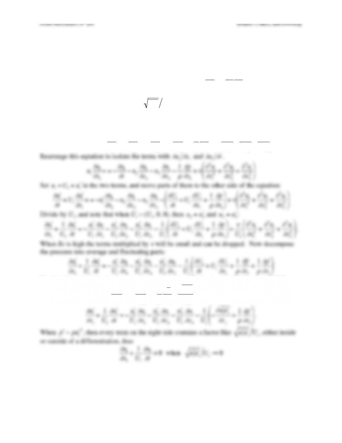
Rearrange this equation to isolate the terms with
∂
u
1
∂
x1
and
∂
u
1
∂
t
.
The first three terms inside the parentheses can be simplified using the “1”-direction RANS
equation for this situation:
∂
U1
∂
t+U1
∂
U1
∂
x1
=−1
ρ
∂
p
∂
x1
−
∂
%
u
1%
u
j
∂
xj
,
∂
#
u
1
∂
x1
+1
U1
∂
#
u
1
∂
t=−#
u
1
U1
∂
u1
∂
x1
−#
u
2
U1
∂
u1
∂
x2
−#
u
3
U1
∂
u1
∂
x3
−1
U1
−
∂
#
u
1#
u
j
∂
xj
+1
ρ
∂
#
p
∂
x1
&
‘
(
(
)
*
+
+
.
When
“
p ~
ρ
“
u
1
2
, then every term on the right side contains a factor like
“
u
i“
u
iU1
, either inside
or outside of a differentiation, thus
∂
u
1
∂
x1
+1
U1
∂
u
1
∂
t≅0
when
“
u
i“
u
iU1→0
Fluid Mechanics, 6th Ed. Kundu, Cohen, and Dowling
Exercise 12.12. a) Starting from (12.33), derive (12.34) via an appropriate process of Reynolds
decomposition and ensemble averaging.
b) Determine an equation for the scalar fluctuation energy =
1
2“
Y 2
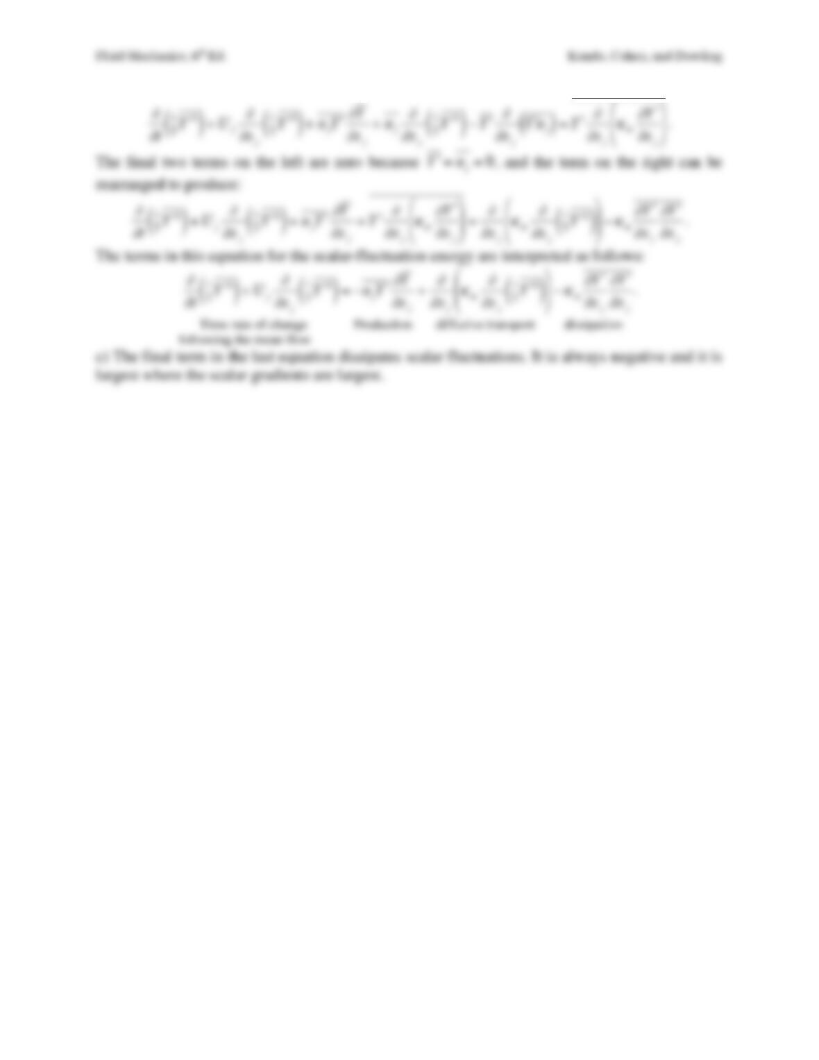
, one half the scalar variance.
c) When the scalar variance goes to zero, the fluid is well mixed. Identify the term in the
equation from part b) that dissipates scalar fluctuation energy.
Solution 12.12. a) First simplify (12.33) for constant density flow by dividing by
ρ
m:
∂
∂
t
ρ
m
˜
Y
( )
+
∂
∂
xj
ρ
m
˜
Y
˜
u
j
( )
=
∂
∂
xj
ρ
m
κ
m
∂
∂
xj
˜
Y
%
&
‘
‘
(
)
*
* →
∂
˜
Y
∂
t+
∂
∂
xj
˜
Y
˜
u
j
( )
=
∂
∂
xj
κ
m
∂
˜
Y
∂
xj
%
&
‘
‘
(
)
*
*
.
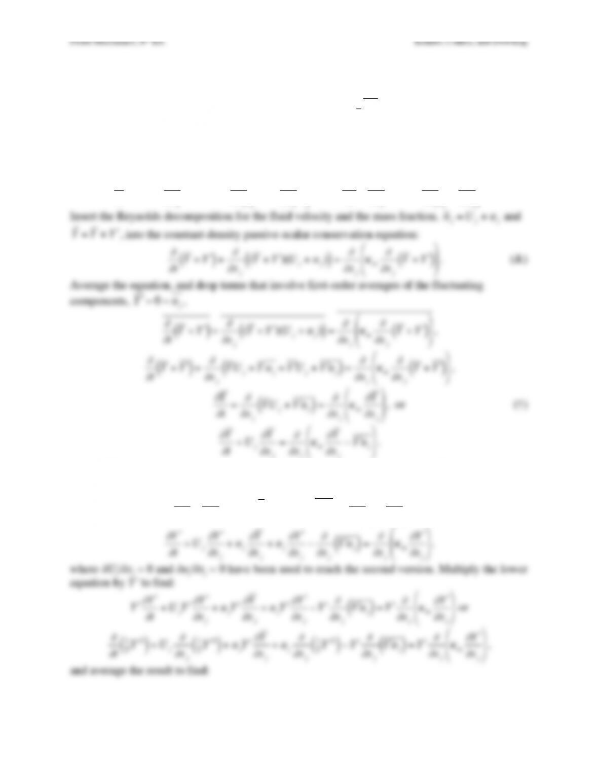
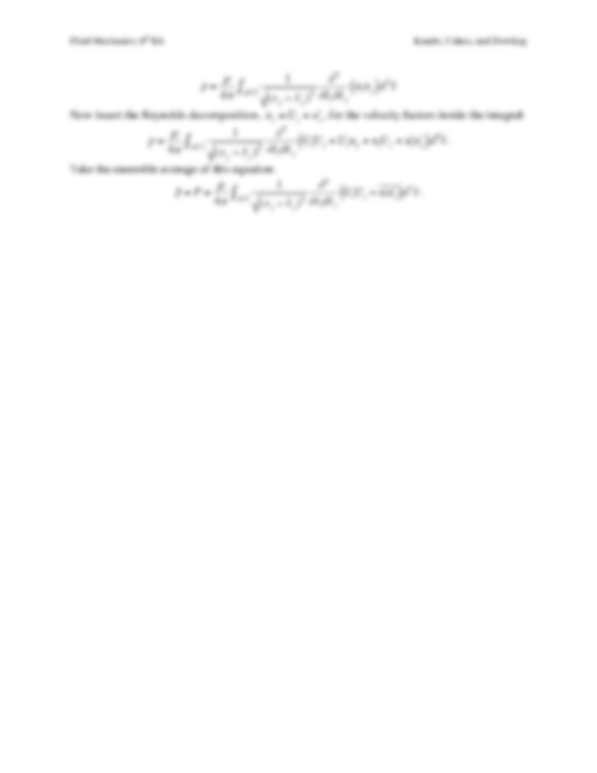
Insert the Reynolds decomposition for the fluid velocity and the mass fraction,
˜
u
j=Uj+uj
and
where ∂Uj/∂xj = 0 has been used to reach the final form which is identical to (12.34).
b) Generate an equation for the scalar fluctuation, by subtracting (†) from (&) to produce:
∂
#
Y
∂
t+
∂
∂
xj
#
Y Uj+Y uj+#
Y uj−#
Y uj
( )
=
∂
∂
xj
κ
m
∂
#
Y
∂
xj
&
‘
(
(
)
*
+
+
, or
∂
#
Y
∂
t+Uj
∂
#
Y
∂
xj
+uj
∂
Y
∂
xj
+uj
∂
#
Y
∂
xj
−
∂
∂
xj
#
Y uj
( )
=
∂
∂
xj
κ
m
∂
#
Y
∂
xj
&
‘
(
(
)
*
+
+
,
where ∂Uj/∂xj = 0 and ∂uj/∂xj = 0 have been used to reach the second version. Multiply the lower
equation by Y´ to find:
“
Y
∂
“
Y
∂
t+Uj“
Y
∂
“
Y
∂
xj
+uj“
Y
∂
Y
∂
xj
+uj“
Y
∂
“
Y
∂
xj
−“
Y
∂
∂
xj
“
Y uj
( )
=“
Y
∂
∂
xj
κ
m
∂
“
Y
∂
xj
&
‘
(
(
)
*
+
+
or
∂
∂
t
1
2#
Y 2
( )
+Uj
∂
∂
xj
1
2#
Y 2
( )
+uj#
Y
∂
Y
∂
xj
+uj
∂
∂
xj
1
2#
Y 2
( )
−#
Y
∂
∂
xj
#
Y uj
( )
=#
Y
∂
∂
xj
κ
m
∂
#
Y
∂
xj
&
‘
(
(
)
*
+
+
,
and average the result to find:
Fluid Mechanics, 6th Ed. Kundu, Cohen, and Dowling
Fluid Mechanics, 6th Ed. Kundu, Cohen, and Dowling
Exercise 12.13. Measurements in an atmosphere at 20 °C show an rms vertical velocity of wrms =
1 m/s and an rms temperature fluctuation of Trms = 0.1°C. If the correlation coefficient is 0.5,
calculate the heat flux
ρ
cpw!
T
.
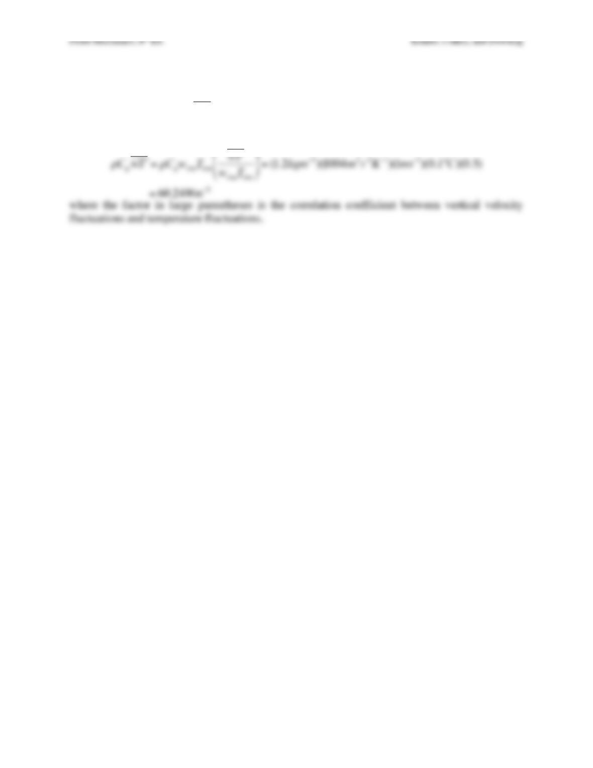
Solution 12.13. The heat flux will be:
ρ
Cpw#
T =
ρ
CpwrmsTrms
w#
T
wrmsTrms
$
%
&
‘
(
) =(1.2kgm−3)(1004m2s−2K−1)(1ms−1)(0.1°C)(0.5)
=60.24Wm−2
where the factor in large parentheses is the correlation coefficient between vertical velocity
fluctuations and temperature fluctuations.
Fluid Mechanics, 6th Ed. Kundu, Cohen, and Dowling
Exercise 12.14. a) Compute the divergence of the constant density Navier-Stokes momentum
equation
∂
ui
∂
t+uj
∂
ui
∂
xj
=−1
ρ
∂
p
∂
xi
+
ν∂
2ui
∂
xj
∂
xj
to determine a Poisson equation for the pressure.
b) If the equation
∂
2G
∂
xj
∂
xj
=
δ
(xj−˜
x j)
has solution:
G(xj,˜
x j)=−1
4
π
(xj−˜
x j)2
, then use the
result from part a) to show that:
P(xj)=
ρ
4
π
1
(xj−!
xj)2
!
x
∫
∂
2
∂
!
xj
∂
!
xi
UiUj+uiuj
( )
d3!
x
in a turbulent
flow.
Solution 12.14. a) Start with
∂
ui
∂
t+uj
∂
ui
∂
xj
=−1
ρ
∂
p
∂
xi
+
ν∂
2ui
∂
xj
∂
xj
and take the divergence (i.e.
apply
∂
∂
xi
to both sides of the equation). This produces:
∂
∂
t
∂
ui
∂
xi
+
∂
uj
∂
xi
∂
ui
∂
xj
+uj
∂
∂
xj
∂
ui
∂
xi
=−1
ρ
∂
2p
∂
xi
∂
xi
+
ν∂
2
∂
xj
∂
xj
∂
ui
∂
xi
The first, third, and final terms are zero in an incompressible flow, leaving
∂
2p
∂
xi
∂
xi
=−
ρ∂
uj
∂
xi
∂
ui
∂
xj
.
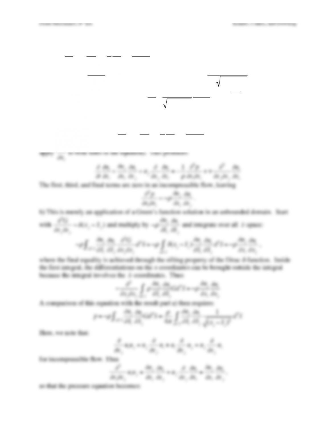
b) This is merely an application of a Green’s function solution in an unbounded domain. Start
with
∂
2G
∂
xj
∂
xj
=
δ
(xj−˜
x j)
and multiply by
−
ρ∂
uj
∂
˜
x
i
∂
ui
∂
˜
x j
and integrate over all
˜
x
-space:
−
ρ∂
uj
∂
!
xi
∂
ui
∂
!
xj
all !
x
∫
∂
2G
∂
xj
∂
xj
d3!
x=−
ρ δ
(xj−!
xj)
∂
uj
∂
!
xi
∂
ui
∂
!
xj
d3!
x
all !
x
∫=−
ρ∂
uj
∂
xi
∂
ui
∂
xj
,
where the final equality is achieved through the sifting property of the Dirac
δ
-function. Inside
the first integral, the differentiations on the x-coordinates can be brought outside the integral
because the integral involves the
˜
x
-coordinates. Thus:
−
∂
2
∂
xj
∂
xj
ρ∂
uj
∂
!
xi
∂
ui
∂
!
xj
all !
x
∫Gd3!
x=−
ρ∂
uj
∂
xi
∂
ui
∂
xj
A comparison of this equation with the result part a) then requires:
p=−
ρ∂
uj
∂
!
xi
∂
ui
∂
!
xj
all !
x
∫Gd3!
x=
ρ
4
π
∂
uj
∂
!
xi
∂
ui
∂
!
xj
all !
x
∫1
(xj−!
xj)2d3!
x
Here, we note that:
∂
∂
xj
uiuj=uj
∂
∂
xj
ui+ui
∂
∂
xj
uj=uj
∂
∂
xj
ui
for incompressible flow. Thus
∂
2
∂
xi
∂
xj
uiuj=
∂
uj
∂
xi
∂
ui
∂
xj
+uj
∂
∂
xj
∂
ui
∂
xi
=
∂
uj
∂
xi
∂
ui
∂
xj
,
so that the pressure equation becomes:
Fluid Mechanics, 6th Ed. Kundu, Cohen, and Dowling
Fluid Mechanics, 6th Ed. Kundu, Cohen, and Dowling
Exercise 12.15. Starting with the RANS momentum equation (12.30), derive the equation for the
kinetic energy of the average flow field (12.46).
Solution 12.15. Start with the definition:
E≡1
2UiUi
, and the RANS equation for Ui:
∂
Ui
∂
t+Uj
∂
Ui
∂
xj
=−1
ρ
∂
p
∂
xi
−g1−
α
T −T0
( )
[ ]
δ
i3+
ν∂
Ui
∂
xj
∂
xj
−
∂
∂
xj
(
u
i(
u
j
.
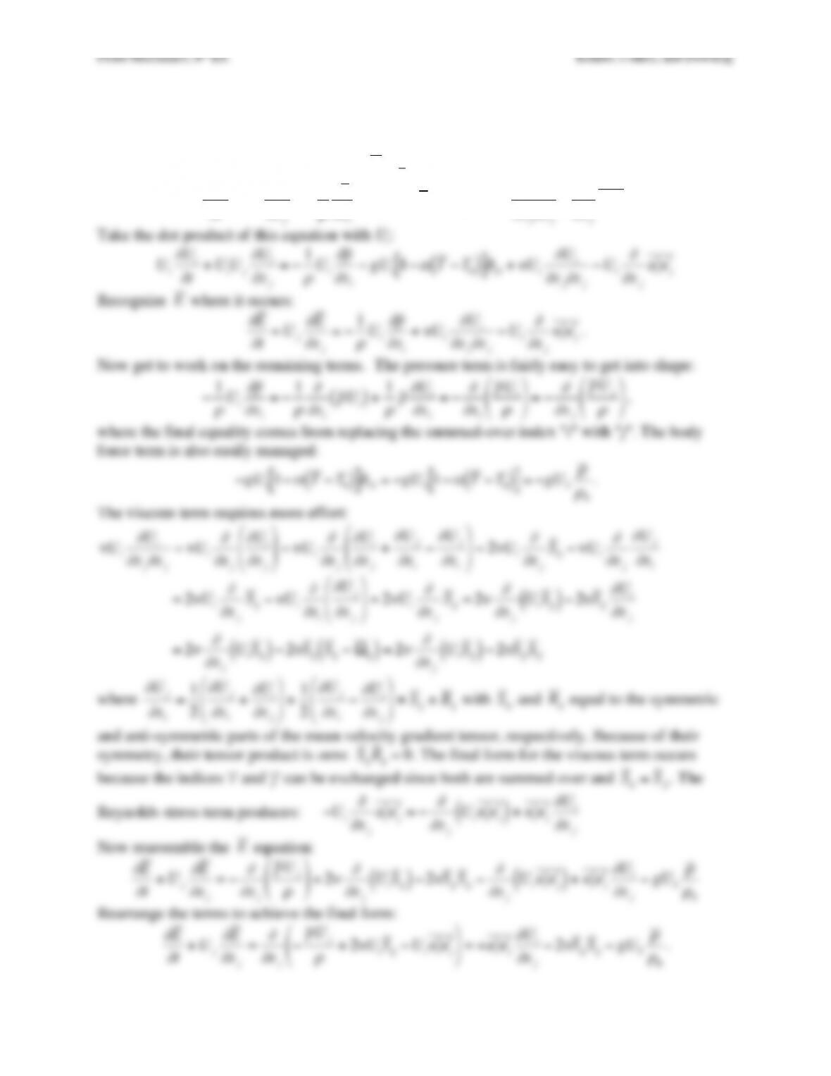
Take the dot product of this equation with Ui:
Fluid Mechanics, 6th Ed. Kundu, Cohen, and Dowling