Fluid Mechanics, 6th Ed. Kundu, Cohen, and Dowling
d
dr
d
dr +1
r
“
#
$ %
&
‘ −K2−
ω
“
#
$
%
&
‘
v=u
,
where
Ta =−4AB
ν
2R2
2=4Ω1
2R
1
4
ν
2
(1−
µ
) 1−
µη
2
( )
2
2
,
κ
=−A
B
R2
2=1−
µη
2
1−
µ
,
µ
=Ω2
Ω1
,
η
=R
1
R2
,
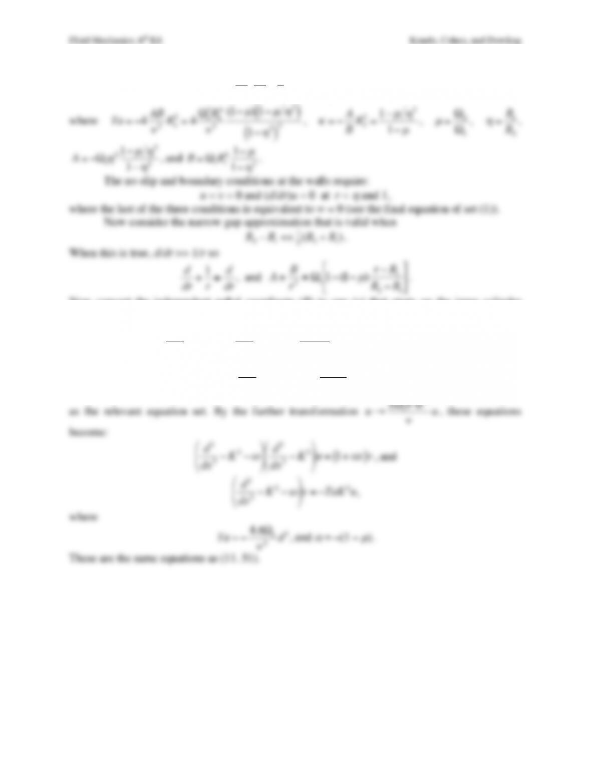
Now convert the independent radial coordinate (R) to one (x) that starts on the inner cylinder
using the gap dimension,
d=R2−R
1
, as the length scale, and let k = K/d, and w =
σ
d2/
ν
to find:
d2
dx 2−K2−
ω
$
%
&
‘
(
)
d2
dx 2−K2
$
%
&
‘
(
)
u=2Ω1d4
ν
K21−(1−
µ
)x
( )
v
, and
d2
dx 2−K2−
ω
$
%
&
‘
(
)
v=2Ad4
ν
u
,
as the relevant equation set. By the further transformation
u→2Ω1d2K4
ν
u
, these equations
Fluid Mechanics, 6th Ed. Kundu, Cohen, and Dowling
Exercise 11.9. Consider the centrifugal instability problem of Section 11.6. From (11.51) and
(11.53), the eigenvalue problem for determining the marginal state (
σ
= 0) is
d2dR2−k2
( )
2ˆ
u
R=(1+
α
x)ˆ
u
ϕ
,
d2dR2−k2
( )
2ˆ
u
ϕ
=−Tak2ˆ
u
R
, (11.92,93)
with
ˆ
u
R=dˆ
u
RdR =ˆ
u
ϕ
=0
at x = 0 and 1. Conditions on
ˆ
u
ϕ
are satisfied by assuming solutions
of the form
ˆ
u
ϕ
=Cmsin(m
π
x)
m=1
∞
∑
. (11.94)
Inserting this into (11.92), obtain an equation for
ˆ
u
R
, and arrange so that the solution satisfies the
four remaining conditions on
ˆ
u
R
. With
ˆ
u
R
determined in this manner and
ˆ
u
ϕ
given by (11.94),
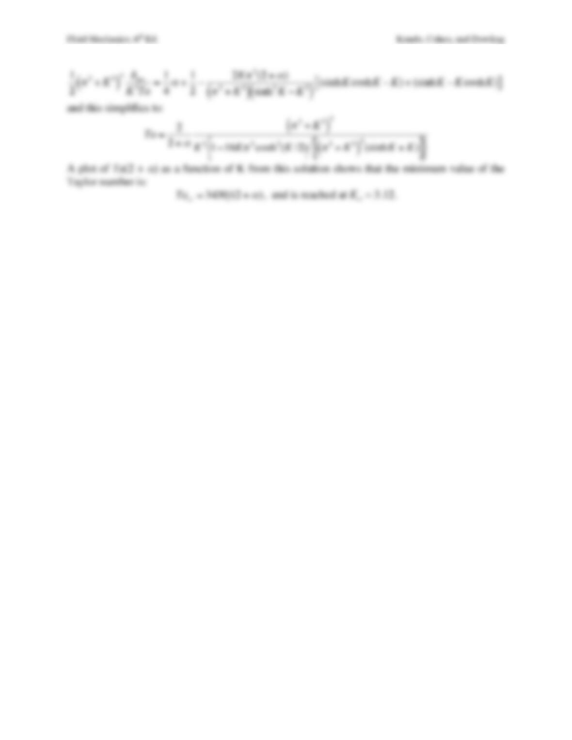
(11.93) leads to an eigenvalue problem for Ta(k). Following Chandrasekhar (1961, p. 300), show
that the minimum Taylor number is given by (11.54) and is reached at kcr = 3.12.
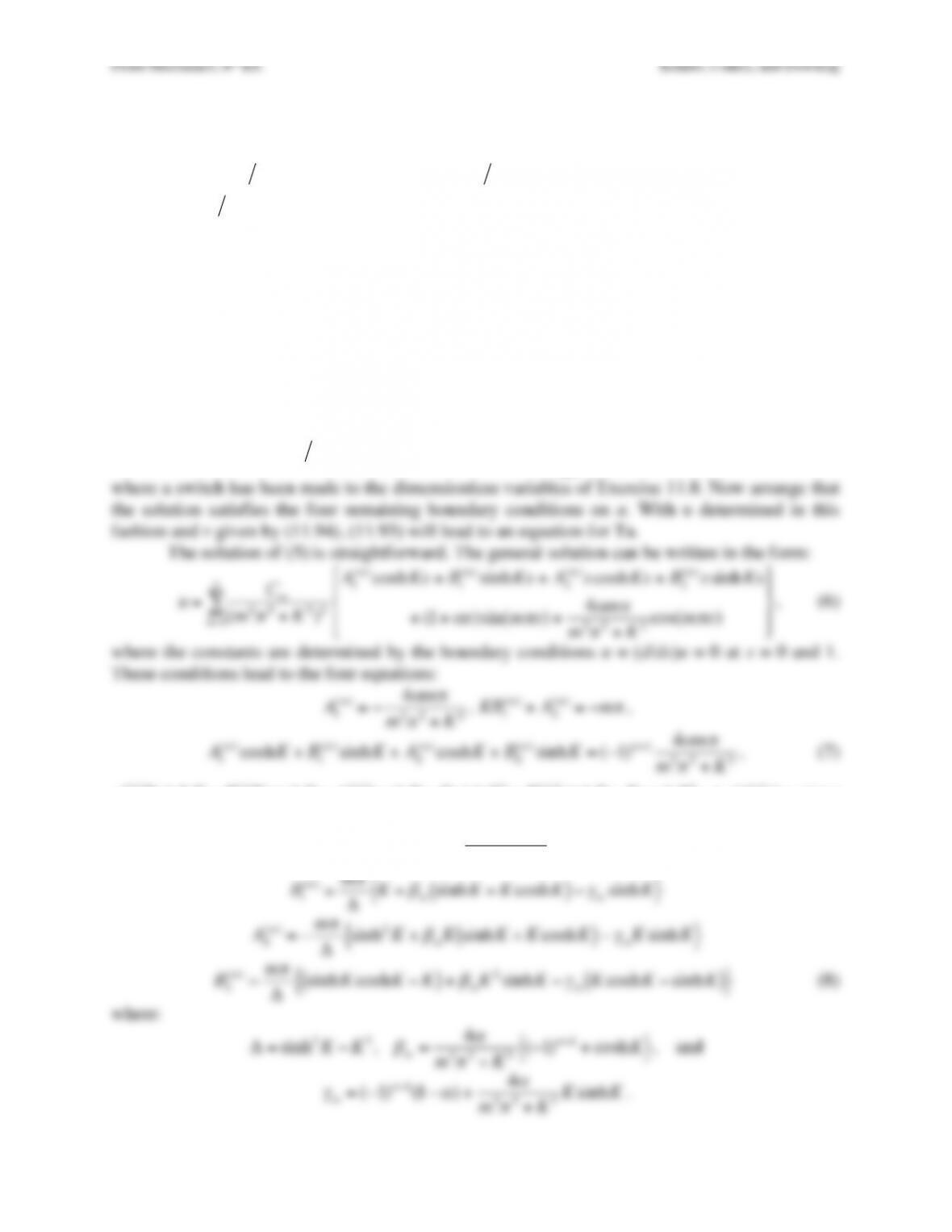
Solution 11.9. Continuing the effort from Exercise 11.8, insert (11.94) into (11.92) to find:
d2dx 2−K2
( )
2u=(1+
α
x)v=(1+
α
x)Cmsin(m
π
x)
m=1
∞
∑
, (5)
where a switch has been made to the dimensionless variables of Exercise 11.8. Now arrange that
α
m
π
A
1
(m)=−4
m2
π
2+K2
,
KB
1
(m)+A2
(m)=−m
π
,
A
1
(m)KsinhK+B
1
(m)KcoshK+A2
(m)coshK+KsinhK
( )
+B2
(m)sinhK+KcoshK
( )
=(−1)m+1(1+
α
)m
π
The solution of these equations is:
A
1
(m)=−4
α
m
π
m2
π
2+K2
B
1
(m)=m
π
Δ
K+
β
msinhK+KcoshK
( )
−
γ
msinhK
{ }
A2
(m)=−m
π
Δsinh2K+
β
mKsinhK+KcoshK
( )
−
γ
mKsinhK
{ }
B2
(m)=m
π
ΔsinhKcoshK−K
( )
+
β
mK2sinhK−
γ
mKcoshK−sinhK
( )
{ }
(8)
where:
Δ=sinh2K−K2
,
β
m=4
α
m2
π
2+K2(−1)m+1+coshK
{ }
, and
γ
m=(−1)m+1(1−
α
)+4
α
m2
π
2+K2KsinhK
.
Fluid Mechanics, 6th Ed. Kundu, Cohen, and Dowling
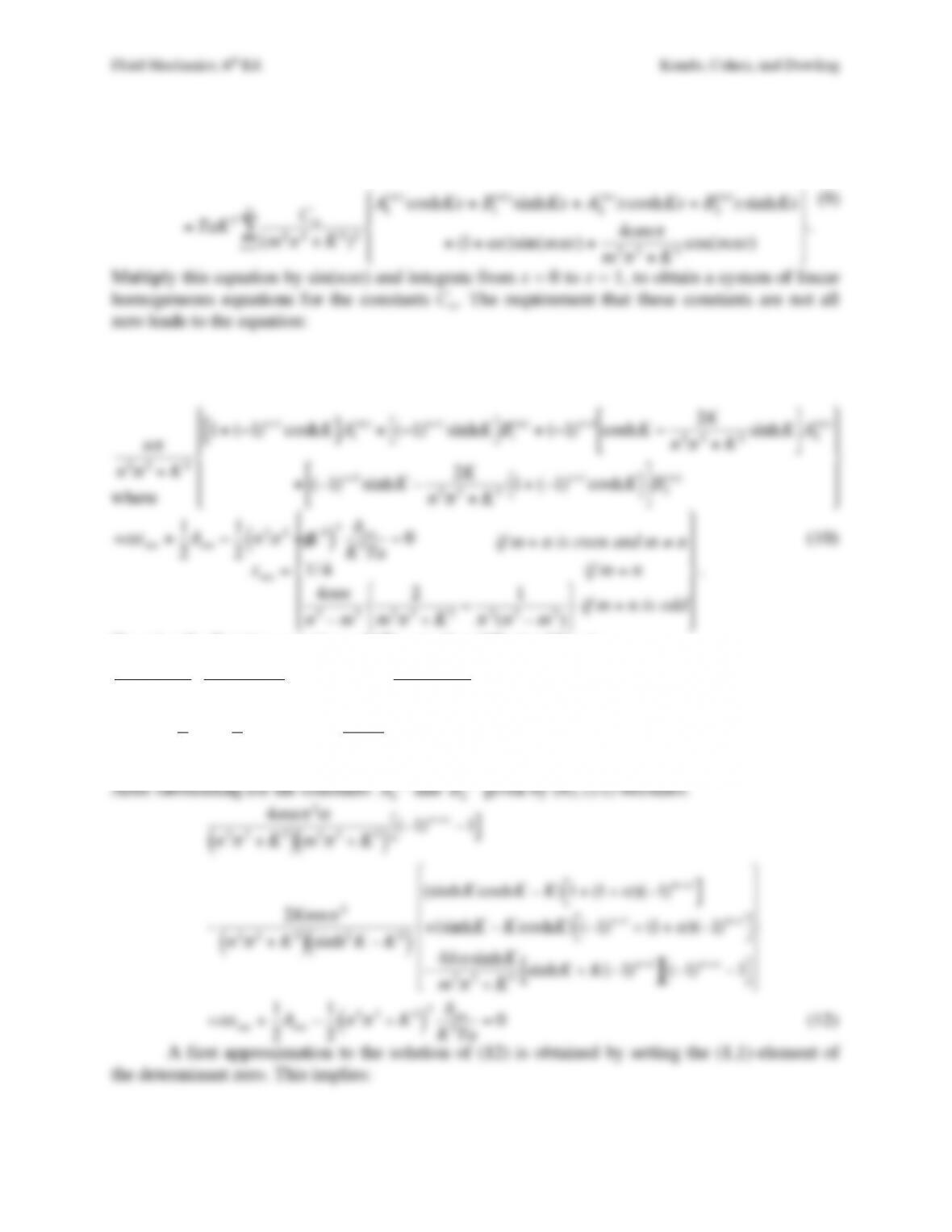
Substituting u from (6) and v from (11.94) into (11.93) produces:
Cnn2
π
2+K2
( )
n=1
∞
∑sin n
π
x
=TaK 2Cm
(m2
π
2+K2)2
A
1
(m)coshKx +B
1
(m)sinhKx +A2
(m)xcoshKx +B2
(m)xsinhKx
+(1+
α
x)sin(m
π
x)+4
α
m
π
m2
π
2+K2cos(m
π
x)
&
‘
(
)
(
*
+
(
,
(
m=1
∞
∑.
(9)
Multiply this equation by sin(nπx) and integrate from x = 0 to x = 1, to obtain a system of linear
homogeneous equations for the constants Cm. The requirement that these constants are not all
zero leads to the equation:
n
π
n2
π
2+K2
1+(−1)n+1coshK
[ ]
A
1
(m)+(−1)n+1sinhK
[ ]
B
1
(m)+(−1)n+1coshK−2K
n2
π
2+K2sinhK
$
%
& ‘
(
)
A2
(m)
+ (−1)n+1sinhK−2K
n2
π
2+K21+(−1)n+1coshK
{ }
$
%
& ‘
(
)
B2
(m)
*
+
,
,
–
,
,
.
/
,
,
0
,
,
+
α
xnm +1
2
δ
nm −1
2
n2
π
2+K2
( )
3
δ
nm
K2Ta =0 (10)
where
xnm =
0 if m+n is even and m≠n
1/ 4 if m=n
4nm
n2−m2
2
m2
π
2+K2−1
π
2(n2−m2)
%
&
‘
(
)
*
if m+n is odd
%
&
+
+
‘
+
+
(
)
+
+
*
+
+
.
On using the first two equations of (7), equation (10) simplifies to:
n
π
n2
π
2+K2
4m
πα
m2
π
2+K2(−1)m+n−1
[ ]
−2K
n2
π
2+K2(−1)n+1A2
(m)sinhK+(−1)n+1B2
(m)coshK+B2
(m)
[ ]
%
&
‘
(
)
*
+
α
xnm +1
2
δ
nm −1
2
n2
π
2+K2
( )
3
δ
nm
K2Ta =0 (11)
After substituting for the constants
A2
(m)
and
B2
(m)
given by (8), (11) becomes:
Fluid Mechanics, 6th Ed. Kundu, Cohen, and Dowling
Fluid Mechanics, 6th Ed. Kundu, Cohen, and Dowling
Exercise 11.10. For a Kelvin–Helmholtz instability in a continuously stratified ocean, obtain a
globally integrated energy equation in the form
1
2
d
dt u2+w2+g2
ρ
2
ρ
0
2N2
( )
dV =−uw
∂
U
∂
z
∫∫ dV
.
(As in Figure 11.25, the integration in x takes place over an integer number of wavelengths.)
Discuss the physical meaning of each term and the mechanism of instability.
Solution 11.10. From (11.57), multiplying the perturbation equations for the Kelvin-Helmholtz
instability by u, w, and
g2
ρ ρ
0
2N2
and add them together
u
∂
u
∂
t+U
∂
u
∂
x+w
∂
U
∂
z+1
ρ
0
∂
p
∂
x
$
%
&
‘
(
) +w
∂
w
∂
t+U
∂
w
∂
x+
ρ
ρ
0
g+1
ρ
0
∂
p
∂
z
$
%
&
‘
(
) +g2
ρ
ρ
0
2N2
∂ρ
∂
t+U
∂ρ
∂
x−
ρ
0wN2
g
$
%
&
‘
(
) =0
.
This produces:
∂
∂
t+U
∂
∂
x
#
$
% &
‘
( u2
2+w2
2+g2
ρ
2
2
ρ
0
2N2
#
$
%
&
‘
( +uw
∂
U
∂
z+1
ρ
0
∂
p
∂
x+
∂
p
∂
z
#
$
% &
‘
( =0
The final term can be rewritten:
∂
∂
t+U
∂
∂
x
#
$
% &
‘
( u2
2+w2
2+g2
ρ
2
2
ρ
0
2N2
#
$
%
&
‘
( +uw
∂
U
∂
z+1
ρ
0
∂
(pu)
∂
x+
∂
(pw)
∂
z
#
$
% &
‘
( −p
∂
u
∂
x+
∂
w
∂
z
#
$
% &
‘
( =0
.
After global integration over an integer number of x-direction wavelengths, the terms involving
U(∂/∂x) will be zero, and the third term, which is equal to
ρ
0
−1∇ ⋅ (pu)dV
∫
, transforms into a
surface integral,
ρ
0
−1pu⋅ndA
∫
, which vanishes because no flow crosses the channel walls and an
there is an equal in-flux and out-flux across the open boundaries on the CV (see Figure 11.25).
The last term vanishes because of the continuity equation. Thus, the resulting CV equation is:
1
2
d
dt u2+w2+g2
ρ
2
ρ
0
2N2
( )
dV =−uw
∂
U
∂
z
∫∫ dV
.
Fluid Mechanics, 6th Ed. Kundu, Cohen, and Dowling
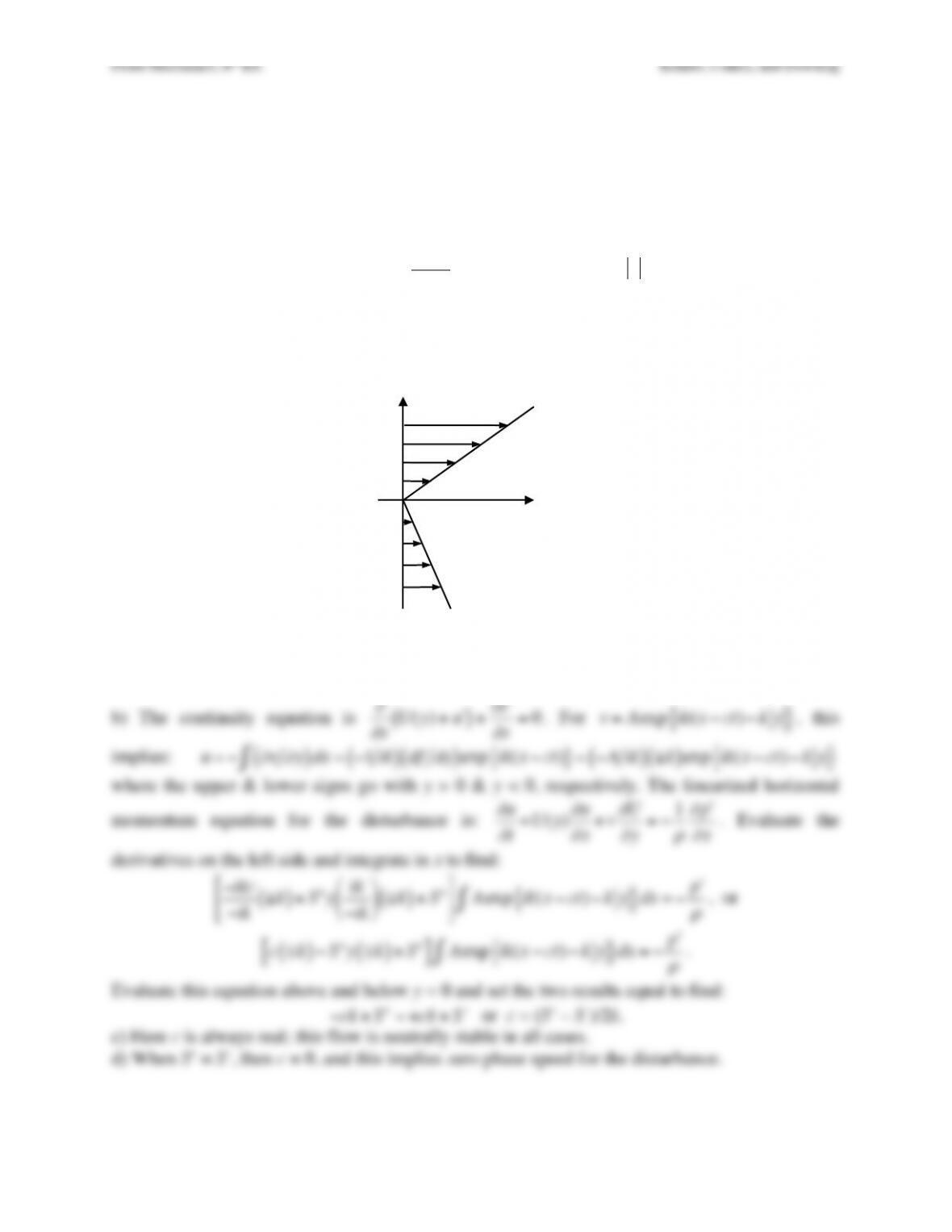
Exercise 11.11. In two-dimensional (x,y)-Cartesian coordinates, consider the inviscid stability of
horizontal parallel shear flow defined by two linear velocity gradients:
U(y)=S+y for y>0
S−y for y≤0
$
%
&
‘
(
)
,
where S+ and S– are real constants. Assume an infinitesimal velocity perturbation with vertical
component
v=f(y)exp ik(x−ct)
{ }
, where k is positive real but
ω
may be complex.
a) Use the Rayleigh equation
!!
f−k2f−f!!
U
U−c=0
with
f(y)→0
as
y→ ∞
to find f(y).
b) Require the pressure perturbation associated with v to be continuous across y = 0, and
determine a single equation for the disturbance phase speed c in terms of the other parameters.
c) For what values of S+, S–, and k, is this flow stable, unstable, or neutrally stable?
d) What is special about the case S+ = S–?
Solution 11.11. a) Here d2U/dy2 = 0, so the Rayleigh equation simplifies to d2f/dy2 – k2f = 0
which has solutions A±exp(±ky). To satisfy the given boundary conditions for k positive & real,
the decaying exponential must be chosen for y > 0 and y < 0, so f(y) = Aexp(–k|y|).
b) The continuity equation is
∂
∂
xU(y)+#
u
( )
+
∂
#
v
∂
x=0
. For
v=Aexp ik(x−ct)−k y
{ }
, this
x!
y!U(y)!
Fluid Mechanics, 6th Ed. Kundu, Cohen, and Dowling
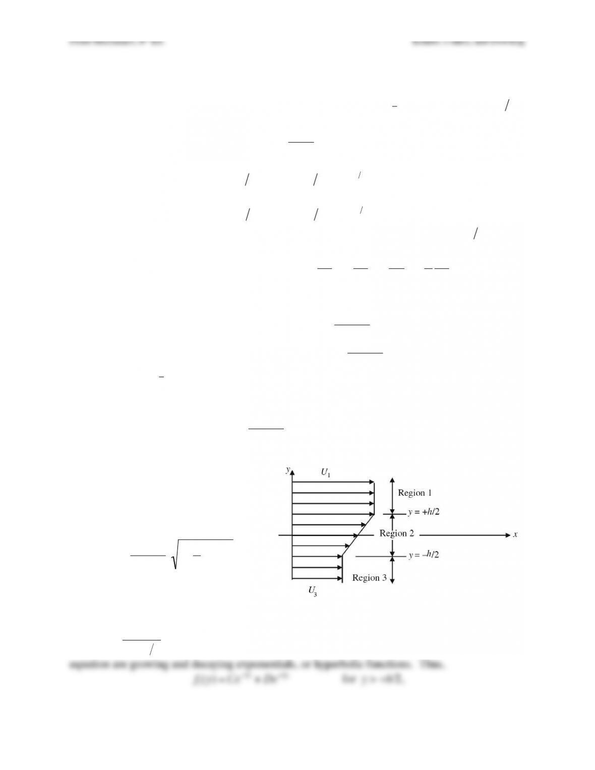
Exercise 11.12. Consider the inviscid stability of a constant vorticity layer of thickness h
between uniform streams with flow speeds U1 and U3. Region 1 lies above the layer, y > h/2
with U(y) = U1. Region 2 lies within the layer, |y| ≤ h/2,
U(y)=1
2(U1+U3)+(U1−U3)y h
( )
.
Region 3 lies below the layer, y < –h/2 with U(y) = U3.
a) Solve the Rayleigh equation,
“ “
f −k2f−f“ “
U
U−c=0
, in each region, then use appropriate
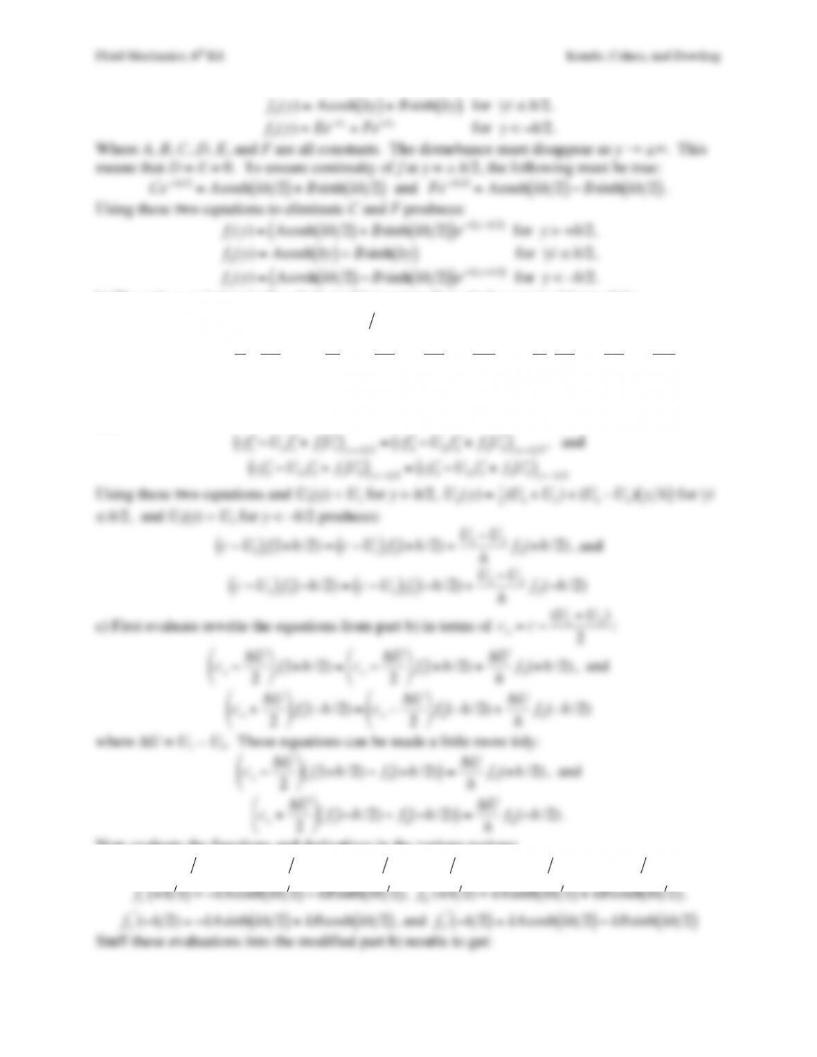
boundary and matching conditions to obtain:
f1(y)=Acosh kh 2
( )
+Bsinh kh 2
( )
( )
e−k y−h2
( )
for y > +h/2,
f2(y)=Acosh ky
( )
+Bsinh ky
( )
for |y| ≤ h/2,
f3(y)=Acosh kh 2
( )
−Bsinh kh 2
( )
( )
e+k y +h2
( )
for y < –h/2.
where f defines the spatial extent of the disturbance:
“
v =f(y)eik(x−ct )
and
“
u =−“
f ik
( )
eik(x−ct )
,
and A and B are undetermined constants.
b) The linearized horizontal momentum equation is:
∂
#
u
∂
t+U
∂
#
u
∂
x+#
v
∂
U
∂
y=−1
ρ
∂
#
p
∂
x
.
Integrate this equation with respect to x, require the pressure to be continuous at y = ± h/2, and
simplify your results to find two additional constraint equations:
c−U1
( )
#
f
1(+h/2) =c−U1
( )
#
f
2(+h/2) +U1−U3
hf2(+h/2)
, and
c−U3
( )
#
f
3(−h/2) =c−U3
( )
#
f
2(−h/2) +U1−U3
hf2(−h/2)
c) Define
co=c−1
2(U1+U3)
(this is the phase speed of the disturbance waves in a frame of
reference moving at the average speed), and use the results of parts a) and b) to determine a
single equation for co:
co
2=U1−U3
2kh
#
$
% &
‘
(
2
kh −1
( )
2−e−2kh
{ }
[This part of this problem requires patience and algebraic skill.]
d) From the result of part c), co will be
real for kh >> 1 (short wave
disturbances), so the flow is stable or
neutrally stable. However, for kh << 1
(long wave disturbances), use the result
of part c) to show that:
co≅±iU1−U3
2
$
%
& ‘
(
) 1−4
3
kh +…
e) Determine the largest value of kh at
which the flow is unstable.
Solution 11.12. Here
“ “
U =0
in all three regions, so the Rayleigh equation,
“ “
f −k2f−f“ “
U
U−
ω
k=0
, reduces to:
“ “
f −k2f=0
in all three regions. The solutions of this
equation are growing and decaying exponentials, or hyperbolic functions. Thus,
Fluid Mechanics, 6th Ed. Kundu, Cohen, and Dowling
b) The only x-variation in the whole problem enters through the assumed form of the
disturbance:
“
v =f(y)eik(x−ct )
and
“
u =−“
f ik
( )
eik(x−ct )
, so and x-integration is the same as dividing
by +ik. Therefore:
−1
ρ
∂
%
p
∂
xdx
∫=−%
p
ρ
=
∂
%
u
∂
t+U
∂
%
u
∂
x+%
v dU
dy
‘
(
)
*
+
,
∫dx =1
ik
∂
%
u
∂
t+U
∂
%
u
∂
x+%
v dU
dy
‘
(
)
*
+
,
, and
there is no integration constant since the pressure fluctuation must disappear when
“
u
and
“
v
disappear. Now plug in the relationships for
“
u
and
“
v
and require continuity of pressure at y = ±
h/2:
c“
f
1−U1“
f
1+f1“
U
1
( )
y= +h2=c“
f
2−U2“
f
2+f2“
U
2
( )
y= +h2
, and
c“
f
2−U2“
f
2+f2“
U
2
( )
y=−h2=c“
f
3−U3“
f
3+f3“
U
3
( )
y=−h2
Using these two equations and U1(y) = U1 for y > h/2,
U2(y)=1
2(U1+U3)+(U1−U3)y h
( )
for |y|
≤ h/2, and U3(y) = U3 for y < –h/2 produces:
c−U1
( )
#
f
1(+h/2) =c−U1
( )
#
f
2(+h/2) +U1−U3
hf2(+h/2)
, and
c−U3
( )
#
f
3(−h/2) =c−U3
( )
#
f
2(−h/2) +U1−U3
hf2(−h/2)
c) First evaluate rewrite the equations from part b) in terms of
co=c−(U1+U3)
2
:
co−ΔU
2
$
%
& ‘
(
) *
f
1(+h/2) =co−ΔU
2
$
%
& ‘
(
) *
f
2(+h/2) +ΔU
hf2(+h/2)
, and
co+ΔU
2
#
$
% &
‘
( )
f
3(−h/2) =co−ΔU
2
#
$
% &
‘
( )
f
2(−h/2) +ΔU
hf2(−h/2)
where ΔU = U1 – U3. These equations can be made a little more tidy:
co−ΔU
2
$
%
& ‘
(
) *
f
1(+h/2) −*
f
2(+h/2)
( )
=ΔU
hf2(+h/2)
, and
co+ΔU
2
#
$
% &
‘
( )
f
3(−h/2) −)
f
2(−h/2)
( )
=ΔU
hf2(−h/2)
.
Now evaluate the functions and derivatives in the various regions:
f2(+h2) =Acosh kh 2
( )
+Bsinh kh 2
( )
,
f2(−h2) =Acosh kh 2
( )
−Bsinh kh 2
( )
,
f1“+h2
( )
=−kAcosh kh 2
( )
−kBsinh kh 2
( )
,
f2“(+h2) =kAsinh kh 2
( )
+kBcosh kh 2
( )
,
f2“(−h2)=−kAsinh kh 2
( )
+kBcosh kh 2
( )
, and
f3“−h2
( )
=kAcosh kh 2
( )
−kBsinh kh 2
( )
Stuff these evaluations into the modified part b) results to get:
Fluid Mechanics, 6th Ed. Kundu, Cohen, and Dowling
co−ΔU
2
$
%
& ‘
(
) −kA cosh kh 2
( )
−kB sinh kh 2
( )
−kA sinh kh 2
( )
−kB cosh kh 2
( )
( )
=ΔU
h
Acosh kh 2
( )
+Bsinh kh 2
( )
( )
,
and
co+ΔU
2
#
$
% &
‘
( kA cosh kh 2
( )
−kB sinh kh 2
( )
+kA sinh kh 2
( )
−kB cosh kh 2
( )
( )
=ΔU
h
Acosh kh 2
( )
−Bsinh kh 2
( )
( )
.
Start simplifying these by collecting terms while noting that
e±z=cosh(z)±sinh(z)
−kh co−ΔU
2
$
%
& ‘
(
) A+B
( )
e+kh 2=ΔU A cosh kh 2
( )
+Bsinh kh 2
( )
( )
+kh co+ΔU
2
#
$
% &
‘
( A−B
( )
e+kh 2=ΔU A cosh kh 2
( )
−Bsinh kh 2
( )
( )
Isolate A and B in each equation.
kh co−ΔU
2
$
%
& ‘
(
)
e+kh 2+ΔUcosh kh
2
$
%
& ‘
(
)
*
+
,
–
.
/
A+kh co−ΔU
2
$
%
& ‘
(
)
e+kh 2+ΔUsinh kh
2
$
%
& ‘
(
)
*
+
,
–
.
/
B=0
kh co+ΔU
2
#
$
% &
‘
(
e+kh 2− ΔUcosh kh
2
#
$
% &
‘
(
*
+
,
–
.
/
A+−kh co+ΔU
2
#
$
% &
‘
(
e+kh 2+ΔUsinh kh
2
#
$
% &
‘
(
*
+
,
–
.
/
B=0
These are two homogeneous linear algebraic equations. They will have a non-trivial solution
when their determinant is zero.
kh co−ΔU
2
$
%
& ‘
(
)
e+kh 2+ΔUcosh kh
2
$
%
& ‘
(
)
*
+
,
–
.
/
× −kh co+ΔU
2
$
%
& ‘
(
)
e+kh 2+ΔUsinh kh
2
$
%
& ‘
(
)
*
+
,
–
.
/
−
kh co−ΔU
2
$
%
& ‘
(
)
e+kh 2+ΔUsinh kh
2
$
%
& ‘
(
)
*
+
,
–
.
/
×kh co+ΔU
2
$
%
& ‘
(
)
e+kh 2− ΔUcosh kh
2
$
%
& ‘
(
)
*
+
,
–
.
/ =0
The remaining job is nothing less than a straight out algebraic effort. First carefully multiply the
factors in square brackets together.
0=−2k2h2co
2−ΔU
( )
2
4
$
%
&
&
‘
(
)
)
ekh +kh co−ΔU
2
$
%
& ‘
(
)
e+kh 2ΔUsinh kh
2
$
%
& ‘
(
)
−kh co+ΔU
2
$
%
& ‘
(
)
e+kh 2ΔUcosh kh
2
$
%
& ‘
(
) +2ΔU
( )
2sinh kh
2
$
%
& ‘
(
)
cosh kh
2
$
%
& ‘
(
)
+kh co−ΔU
2
$
%
& ‘
(
)
e+kh 2ΔUcosh kh
2
$
%
& ‘
(
) −kh co+ΔU
2
$
%
& ‘
(
)
e+kh 2ΔUsinh kh
2
$
%
& ‘
(
)
Collect and simplify all the terms with hyperbolic functions.
0=−2k2h2co
2−ΔU
( )
2
4
$
%
&
&
‘
(
)
)
ekh +kh co−ΔU
2
$
%
& ‘
(
)
e+khΔU−kh co+ΔU
2
$
%
& ‘
(
)
e+khΔU+2ΔU
( )
2e+kh −e−kh
4
$
%
&
‘
(
)
Merge the two middle terms.
0=−2k2h2co
2−ΔU
( )
2
$
&
‘
)
ekh −kh ΔU
2e+kh +2ΔU
2e+kh −e−kh
$
‘
Fluid Mechanics, 6th Ed. Kundu, Cohen, and Dowling
Fluid Mechanics, 6th Ed. Kundu, Cohen, and Dowling
Exercise 11.13. Consider the inviscid instability of parallel flows given by the Rayleigh equation
(U−c)d2ˆ
v
dy2−k2ˆ
v
#
$
%
&
‘
( −d2U
dy2ˆ
v = 0
, (11.95)
where the y-component of the perturbation velocity is
v=ˆ
v (y)exp ik(x−ct)
{ }
.
(i) Note that this equation is identical to the Rayleigh equation (11.81) for the stream
function amplitude
φ
, as it must because
ˆ
v (y)=−ik
φ
. For a flow bounded by walls at y1
and y2, note that the boundary conditions are identical in terms of
φ
and
ˆ
v
.
(ii) Show that if c is an eigenvalue of (11.95), then so is its conjugate c* = cr – ici. What
aspect of (11.95) allows this result to be valid?
(iii) Let U(y) be antisymmetric, so that U(y) = –U(–y). Demonstrate that if c(k) is an
eigenvalue, then –c(k) is also an eigenvalue. Explain the result physically in terms of the
possible directions of propagation of perturbations in such an antisymmetric flow.
(iv) Let U (y) be symmetric so that U(y) = U(–y). Show that in this case
ˆ
v
is either symmetric
or antisymmetric about y = 0.
[Hint: Letting y → – y, show that the solution
ˆ
v (−y)
satisfies (11.95) with the same
eigenvalue c. Form a symmetric solution
S(y)=ˆ
v (y)+ˆ
v (−y)=S(−y)
, and an antisymmetric
solution
A(y)=ˆ
v (y)−ˆ
v (−y)=−A(−y)
. Then write A[S-eqn] – S[A-eqn] = 0 where S-eqn
indicates the differential equation (11.95) in terms of S. Canceling terms this reduces to (SA# –
AS#)# = 0, where the prime (#) indicates a y-derivative. Integration gives SA# – AS# = 0, where the
constant of integration is zero because of the boundary conditions. Another integration gives S =
bA, where b is a constant of integration. Because the symmetric and antisymmetric functions
cannot be proportional, it follows that one of them must be zero.]
Comments: If v is symmetric, then the cross-stream velocity has the same sign across the
entire flow, although the sign alternates every half wavelength along the flow. This mode is
consequently called sinuous. On the other hand, if v is antisymmetric, then the shape of the jet
expands and contracts along the length. This mode is now generally called the sausage instability
because it resembles a line of linked sausages.
Solution 11.13. (i) Since the stream function is
ψ
=
φ
exp[ik(x – ct)], the cross stream velocity is:
v=−
∂ψ
∂
x=−ik
φ
exp ik(x−ct)
[ ]
=ˆ
v exp ik(x−ct)
[ ]
so that
ˆ
v =−ik
φ
.
Thus,
ˆ
v
and
φ
will satisfy identical equations and boundary conditions.
(ii) The complex conjugate of (11.95) is:
(U−c*)d2ˆ
v
*
dy2−k2ˆ
v
*
#
$
%
&
‘
( −d2U
dy2ˆ
v
*= 0
,
and this equation is identical to (11.95) except that c* replaces c and
ˆ
v
*
replaces
ˆ
v
. The
boundary conditions on
ˆ
v
*
and
ˆ
v
are also identical, namely
ˆ
v
*
=
ˆ
v
= 0 at y1 or y2. Thus, if
ˆ
v
is
an eigenfunction with eigenvalue c for some k, then
ˆ
v
*
is and eigenfunction with eigenvalue c* =
cr – ici for the same k. This property is only possible since (11.95) does not directly involve the
imaginary root i.
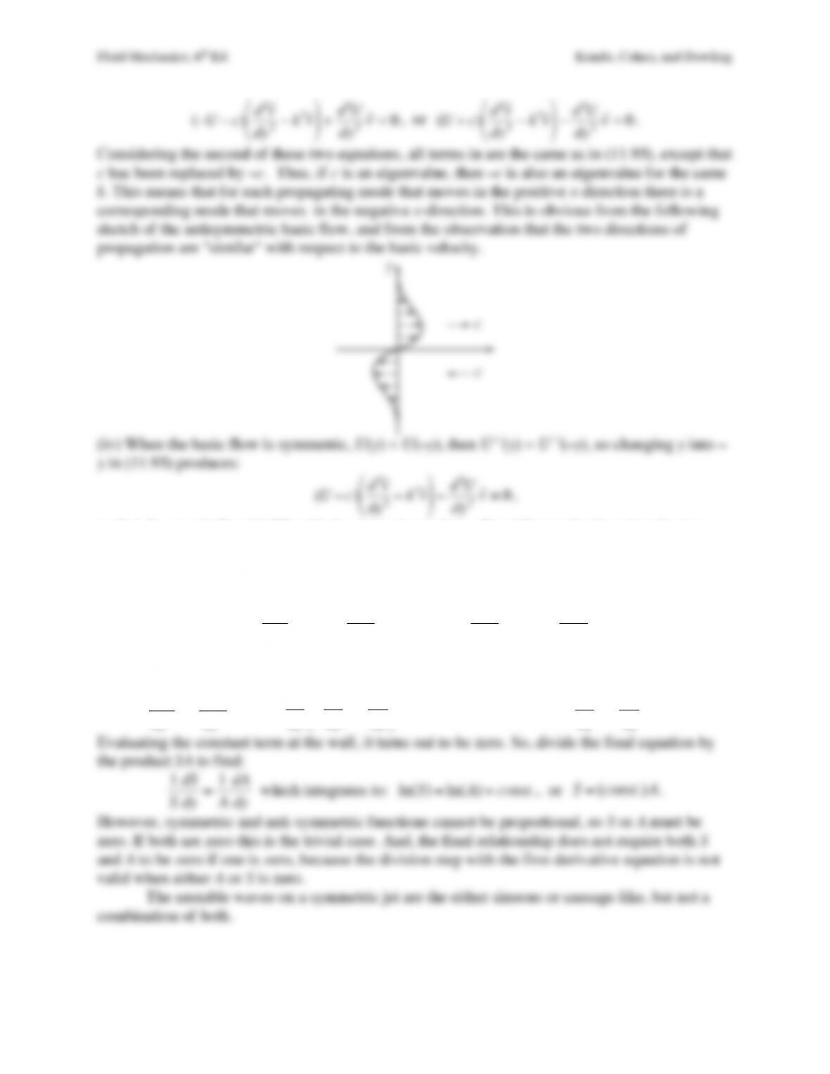
(iii) When the basic flow is antisymmetric, U(y) = –U(–y), so that all derivatives of U change
sign when y is oppositely directed. That is, U´(y) = –U´(–y) and U´´(y) = –U´´(–y), where a prime
denotes a derivative. Changing y into –y, (11.95) becomes:
Fluid Mechanics, 6th Ed. Kundu, Cohen, and Dowling
so that
ˆ
v (−y)
satisfies (11.95) with the same eigenvalue c. By adding and subtracting the two
solutions, we get symmetric and anti-symmetric solutions:
S(y)=ˆ
v (y)+ˆ
v (−y)=S(−y)
and
A(y)=ˆ
v (y)−ˆ
v (−y)=−A(−y)
.
Obviously S and A satisfy the differential equation, therefore:
A(U−c)d2S
dy2−k2S
#
$
%
&
‘
( −d2U
dy2S
)
*
+
,
–
.
−S(U−c)d2A
dy2−k2A
#
$
%
&
‘
( −d2U
dy2A
)
*
+
,
–
. = 0
,
since the contents of both sets of {,]-brackets are zero. Canceling terms and dividing by U – c
leaves:
Ad2S
dy2−Sd2A
dy2= 0
or
d
dy AdS
dy −SdA
dy
#
$
%
&
‘
( = 0
which integrates to
AdS
dy −SdA
dy
=const.
Evaluating the constant term at the wall, it turns out to be zero. So, divide the final equation by
combination of both.
Fluid Mechanics, 6th Ed. Kundu, Cohen, and Dowling
Exercise 11.14. Derive (11.88) starting from the incompressible Navier-Stokes momentum
equation for the disturbed flow:
∂
∂
tUi+ui
( )
+Uj+uj
( )
∂
∂
xj
Ui+ui
( )
=−1
ρ
∂
∂
xi
P+p
( )
+
ν∂
2
∂
xj
∂
xj
Ui+ui
( )
, (11.96)
where Ui and ui represent the basic flow and the disturbance, respectively. Subtract the equation
of motion for the basic state from (11.96), multiply by ui and integrate the result within a
stationary volume having stream-wise control surfaces chosen to coincide with the walls where
no-slip conditions are satisfied or where ui
→
0, and having a length (in the stream-wise
direction) that is an integer number of disturbance wavelengths.
Solution 11.14. The basic flow momentum equation is:
∂
Ui
∂
t+Uj
∂
Ui
∂
xj
=−1
ρ
∂
P
∂
xi
+
ν∂
2Ui
∂
xj
∂
xj
.
Subtracting this from (11.96) produces:
∂
ui
∂
t+uj
∂
Ui
∂
xj
+Uj
∂
ui
∂
xj
+uj
∂
ui
∂
xj
=−1
ρ
∂
p
∂
xi
+
ν∂
2ui
∂
xj
∂
xj
.
Multiply by ui and integrate each term over the CV.
ui
∂
ui
∂
t+uiUj
∂
ui
∂
xj
+uiuj
∂
ui
∂
xj
+uiuj
∂
Ui
∂
xj
=−ui
ρ
∂
p
∂
xi
+ui
ν∂
2ui
∂
xj
∂
xj
&
‘
(
)
*
+
CV
∫dV
. (%)
Consider each term individually.
ui
∂
ui
∂
t
CV
∫dV =
∂
∂
t
1
2
ui
2
$
%
& ‘
(
)
CV
∫dV =d
dt
1
2
ui
2
CV
∫dV
.
Here the final equality follows because the CV is stationary and the volume integration leaves no
spatial dependence.
uiUj
∂
ui
∂
xj
CV
∫dV =1
2Uj
∂
ui
2
∂
xj
+ui
2
∂
Uj
∂
xj
$
%
&
&
‘
(
)
)
CV
∫dV =1
2
∂
(ui
2Uj)
∂
xj
$
%
&
&
‘
(
)
)
CV
∫dV =1
2ui
2Ujnj
CS
∫dA =0
uiuj
∂
ui
∂
xj
CV
∫dV =1
2uj
∂
ui
2
∂
xj
+ui
2
∂
uj
∂
xj
$
%
&
&
‘
(
)
)
CV
∫dV =1
2
∂
(ui
2uj)
∂
xj
$
%
&
&
‘
(
)
)
CV
∫dV =1
2ui
2ujnj
CS
∫dA =0
Here CS is the control surface, and nj are the components of the outward normal vector from the
control surface. And, ∂uj/∂xj = 0 = ∂Uj/∂xj has been used along with Gauss’ theorem, and the fact
that velocity fluctuations are zero on the stream wise control surfaces (no slip), or equal on the
stream-normal control surfaces where nj changes sign between the inlet and the outlet (periodic)
leading to cancellation.
ui
∂
p
∂
xi
CV
∫dV =
∂
(pui)
∂
xi
+p
∂
ui
∂
xi
$
%
&
‘
(
)
CV
∫dV =puini
CS
∫dA =0
.
ui
∂
ui
∂
xj
2
CV
∫dV =
∂
∂
xj
ui
∂
ui
∂
xj
$
%
&
&
‘
(
)
)
CV
∫dV −
∂
ui
∂
xj
∂
ui
∂
xj
CV
∫dV =ui
∂
ui
∂
xj
nj
CS
∫dA −
∂
ui
∂
xj
∂
ui
∂
xj
CV
∫dV =−
∂
ui
∂
xj
∂
ui
∂
xj
CV
∫dV
.
Here again incompressibility, Gauss’ theorem, and the no slip and periodic boundary conditions
lead to the simplifications. Thus, (%) becomes:
d
dt
1
2ui
2
CV
∫dV =−
ρ
uiuj
∂
Ui
∂
xj
CV
∫dV −
ν∂
ui
∂
xj
∂
ui
∂
xj
CV
∫dV
,
which is (11.88).
Fluid Mechanics, 6th Ed. Kundu, Cohen, and Dowling
Exercise 11.15. The process of transition from laminar to turbulent flow may be driven both by
exterior flow fluctuations and nonlinearity. Both of these effects can be simulated with the
simple nonlinear logistic map
xn+1=Axn(1−xn)
and a computer spread-sheet program. Here, xn
can be considered to be the flow speed at the point of interest with A playing the role of the
nonlinearity parameter (Reynolds number), x0 (the initial condition) playing the role of an
external disturbance, and iteration of the equation playing the role of increasing time. The
essential feature illustrated by this problem is that increasing the nonlinearity parameter or
changing the initial condition in the presence of nonlinearity may fully alter the character of the
resulting sequence of xn values. Plotting xn vs. n should aid understanding in parts b) through e).
a) Determine the background solution of the logistic map that occurs when
xn+1=xn
in terms of
A.
Now, get into a spread sheet program, and set up a column that computes
xn+1
for n = 1 to 100 for
user selectable values of x0 and A for 0 < x0 < 1, and 0 < A < 4.
b) For A = 1.0, 1.5, 2.0, 2.9, choose a few different x0’s and numerically determine if the
background solution is reached by n = 100. Is the flow stable for these values of A, i.e. does it
converge toward the background solution?
c) For the slightly larger value, A = 3.2, choose x0 = 0.6875, 0.6874, and 0.6876. Is the flow
stable or oscillatory in these three cases? If it is oscillatory, how many iterations are needed for
it to repeat?
d) For A = 3.5, is the flow stable or oscillatory? If it is oscillatory, how many iterations are
needed for it to repeat? Does any value of x0 lead to a stable solution?
e) For A = 3.9, is the flow stable, oscillatory, or chaotic? Does any value of x0 lead to a stable
solution?
Solution 11.15. a) Setting xn = xn+1 = x in
xn+1=Axn(1−xn)
, produces:
x=Ax(1−x)
. Thus for x
≠ 0, the equilibrium or steady-flow solution for x is
x=1−1A
( )
.
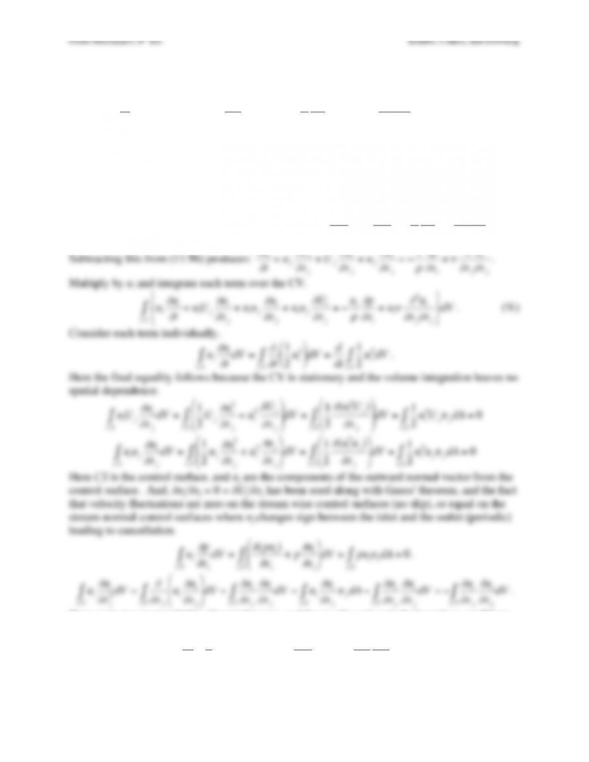
b) For A = 1.0, the solution is not converged but it is heading monotonically toward x = 0. This
Fluid Mechanics, 6th Ed. Kundu, Cohen, and Dowling
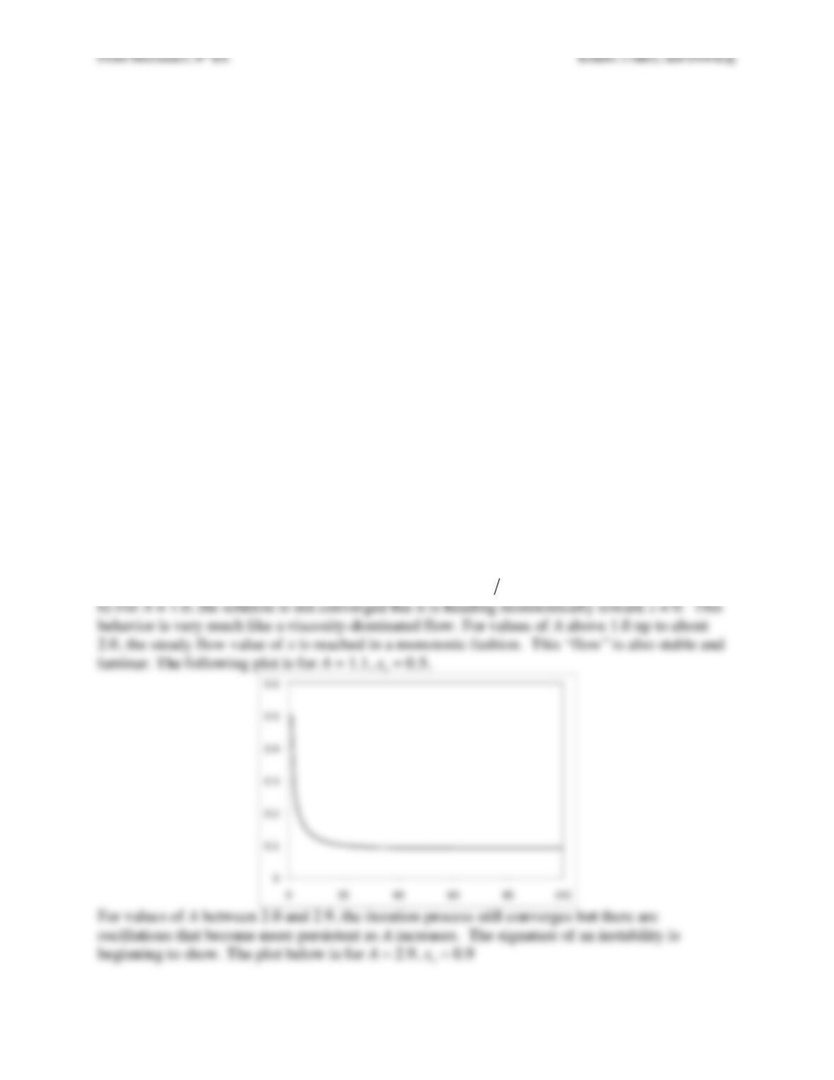
c) For A = 3.2, choose x0 = 0.6875, the equilibrium solution is maintained as shown in the
following plot.
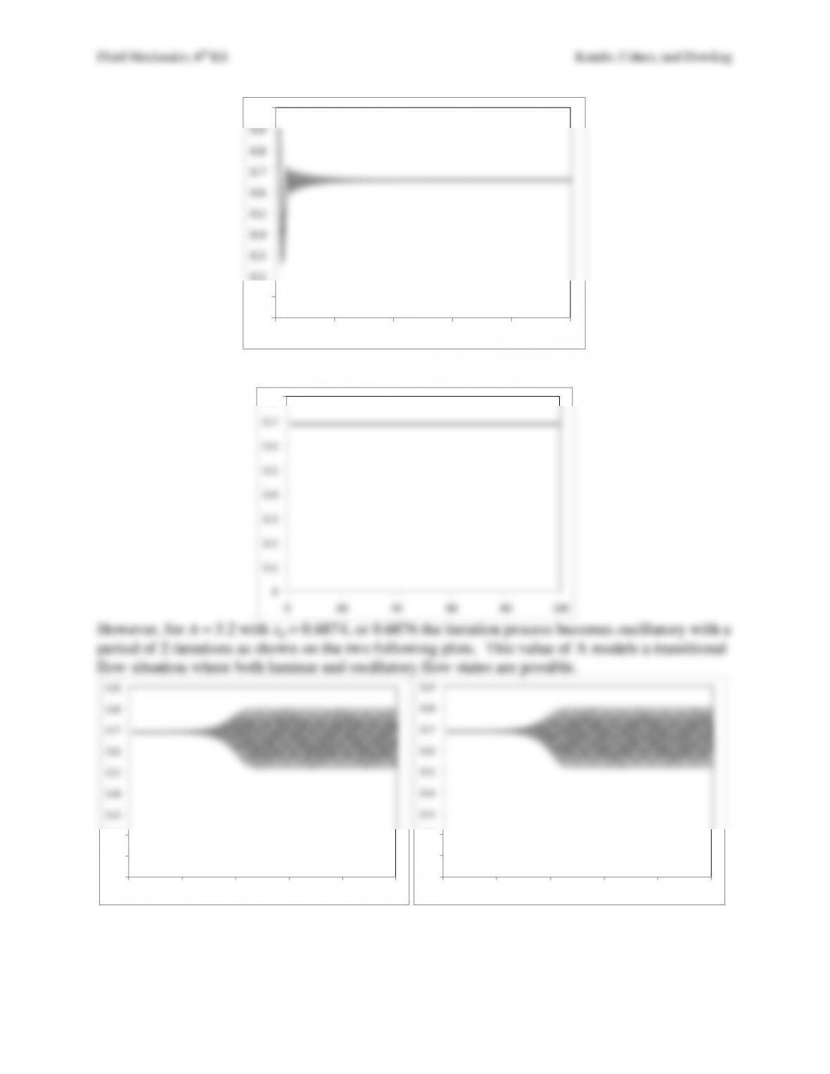
d) For A = 3.5 the flow is always oscillatory no matter what value of x0 is chosen, and the period
is 4 iterations. This “flow” is on its way to becoming turbulent because there are no stable
!”
!#$”
!#%”
!#&”
!#'”
!#(“
!#)”
!#*”
!#+”
!#,”
$”
!” %!” ‘!” )!” +!” $!!”
!”
!#$”
!#%”
!#&”
!#'”
!#(“
!#)”
!#*”
!#+”
!” %!” ‘!” )!” +!” $!!”
!”
!#$”
!#%”
!#&”
!#'”
!#(“
!#)”
!#*”
!#+”
!” %!” ‘!” )!” +!” $!!”
!”
!#$”
!#%”
!#&”
!#'”
!#(“
!#)”
!#*”
!#+”
!” %!” ‘!” )!” +!” $!!”
Fluid Mechanics, 6th Ed. Kundu, Cohen, and Dowling
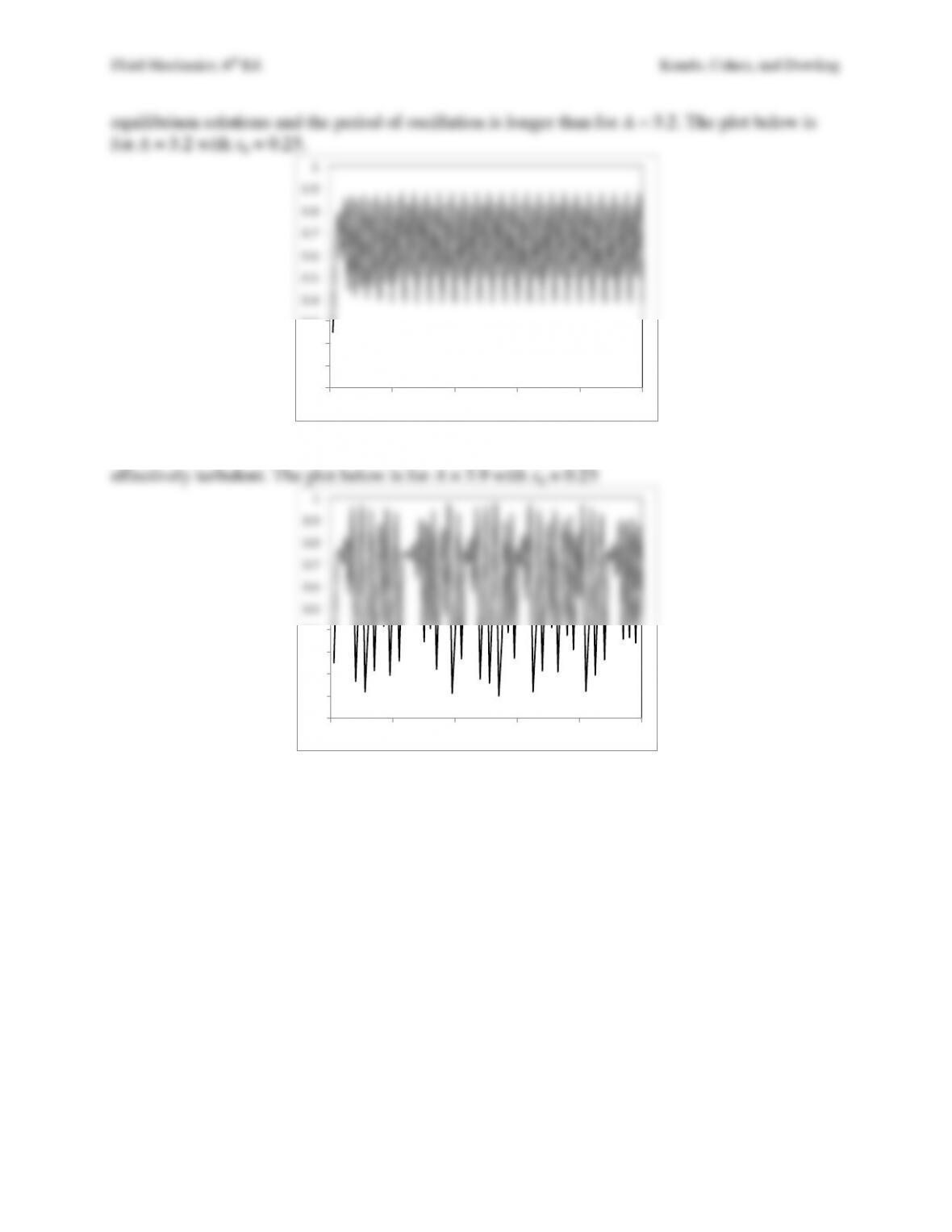
e) For A = 3.9, fluctuations occur no matter what value of x0 is chosen, but these fluctuations are
chaotic and do not repeat; the oscillation period is too large to be defined. This “flow” is
effectively turbulent. The plot below is for A = 3.9 with x0 = 0.25
!”
!#$”
!#%”
!#&”
!#'”
!#(“
!#)”
!#*”
!#+”
!#,”
!” %!” ‘!” )!” +!” $!!”
!”
!#$”
!#%”
!#&”
!#'”
!#(“
!#)”
!#*”
!#+”
!#,”
!” %!” ‘!” )!” +!” $!!”