Fluid Mechanics, 6th Ed. Kundu, Cohen, and Dowling
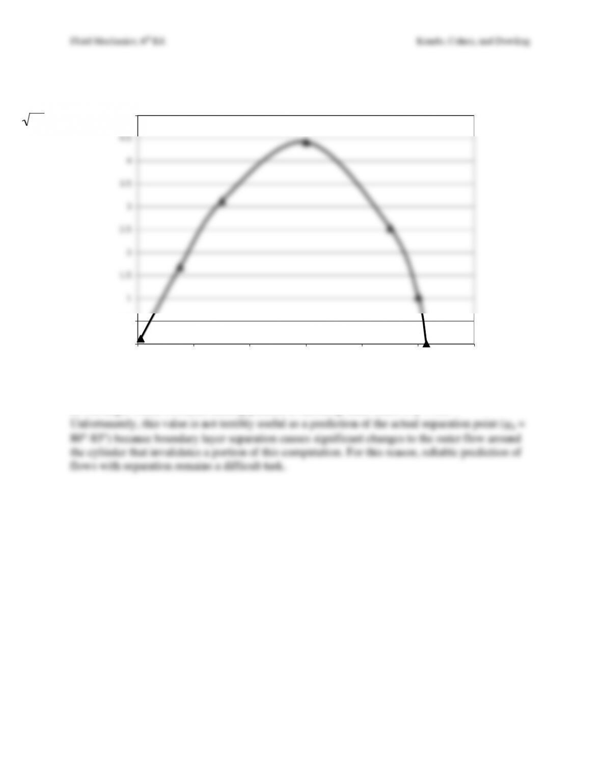
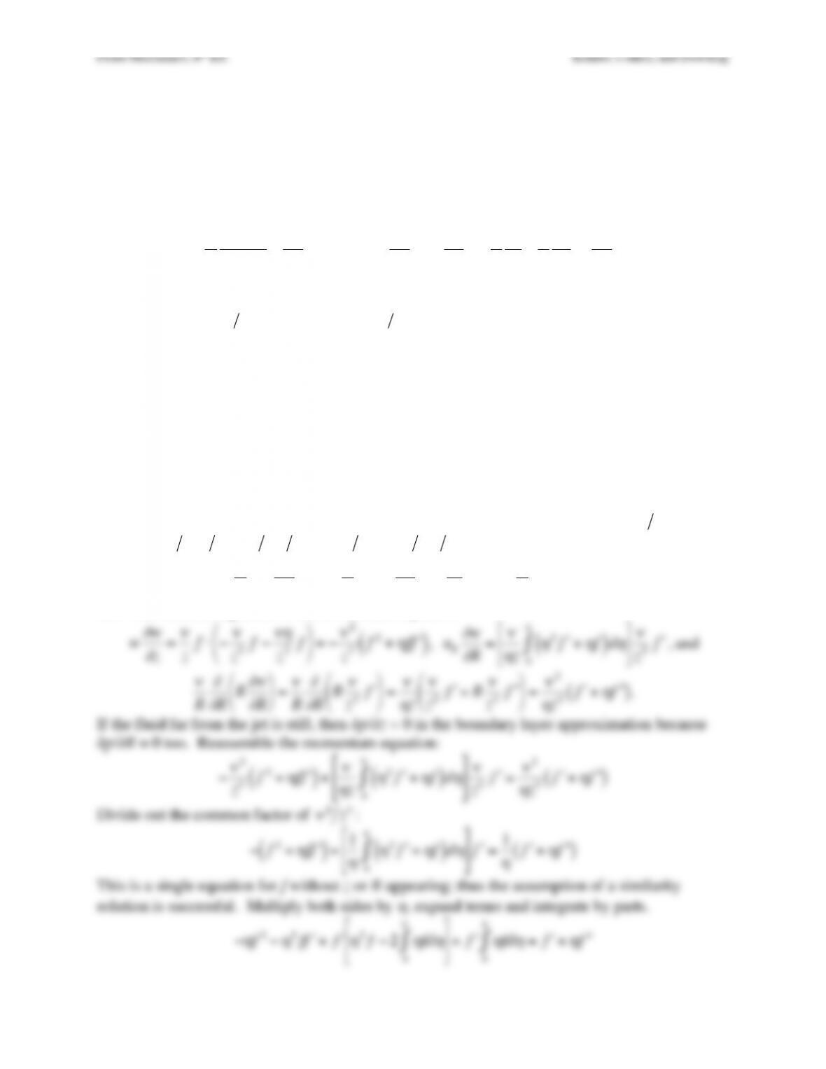
103° -0.089 ~0.0 ~0.0
The maximum surface shear stress is felt at
ϕ
≈ 60°.
c) The angle where Thwaites methog predicts a vanishing shear stress is
ϕ
≈ 103°.
Unfortunately, this value is not terribly useful as a prediction of the actual separation point (
ϕ
s ≈
0
0.5
1
1.5
2
2.5
3
3.5
4
4.5
5
0 20 40 60 80 100 120
angle (degrees)
cfRe
Fluid Mechanics, 6th Ed. Kundu, Cohen, and Dowling
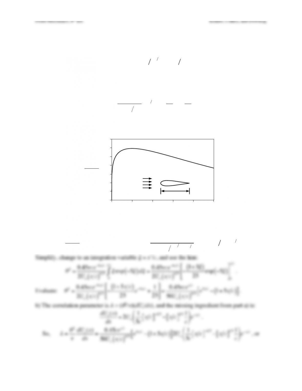
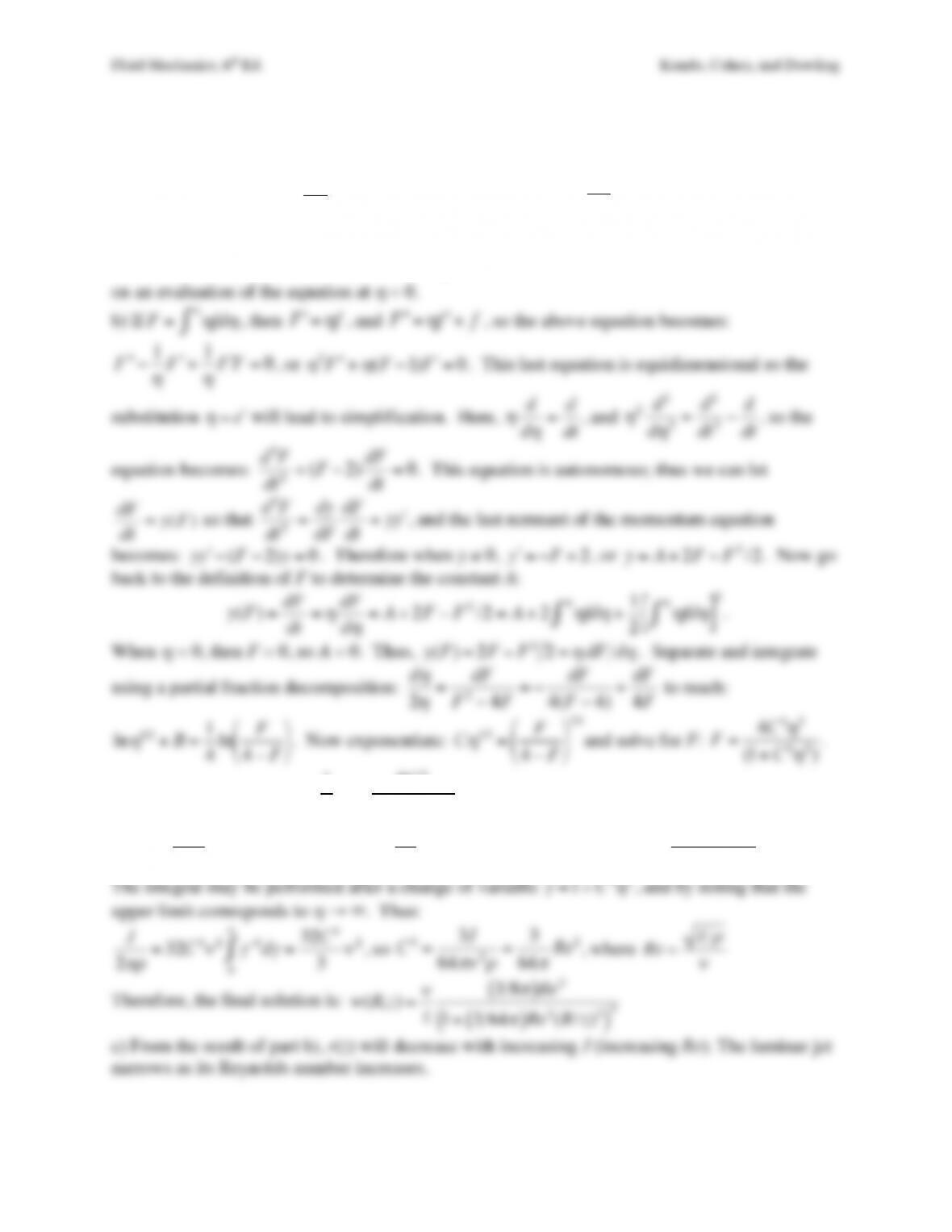
Exercise 10.24. An ideal flow model predicts the following surface velocity for the suction (i.e.
the upper) side of a thin airfoil with chord c placed in a uniform horizontal air stream of speed
Uo:
Ue(x)=2Uox c
[ ]
1 5 exp −x c
( )
.
a) Assuming that x is the coordinate along the foil’s suction surface, use Thwaites method to
estimate the momentum thickness
θ
(x) of the laminar boundary layer that develops on this
surface.
b) Using the results of part a) show that the correlation parameter
λ
is given by:
λ
=0.45
125 x c
( )
2e5x c −1−5x
c
“
#
$%
&
‘1−5x
c
“
#
$%
&
‘
c) Does Thwaites method predict boundary layer separation in the range 1/5 < x/c < 1?
d) If a laminar boundary layer is predicted to separate from the surface of this airfoil, suggest at
least two changes that could be made to the foil that would tend to prevent separation.
Solution 10.24. a) The boundary layer is launched from a stagnation point, so the basic Thwaites
formula is:
θ
2=0.45
ν
Ue
6Ue
5dx
0
x
∫
, or in this case:
θ
2=0.45
ν
26Uo
6x c
( )
6 5 e−6x c
25Uo
5“
x c
( )
e−5“
x c d“
x
0
x
∫
.
Simplify, change to an integration variable
ξ
= x´/c, and use the hint:
0″
0.2″
0.4″
0.6″
0.8″
1″
1.2″
1.4″
0″ 0.2″ 0.4″ 0.6″ 0.8″ 1″
x/c!
Ue(x)
Uo
!
!
!
!
Uo!
c!
Fluid Mechanics, 6th Ed. Kundu, Cohen, and Dowling
Fluid Mechanics, 6th Ed. Kundu, Cohen, and Dowling
Exercise 10.25. An incompressible viscous fluid flows steadily in a large duct with constant
cross sectional area Ao and interior perimeter b. A laminar boundary layer develops on the duct’s
sidewalls. At x = 0, the fluid velocity in the duct is uniform and equal to Uo, and the boundary
layer thickness is zero. Assume the thickness of the duct-wall boundary layer is small compared
to Ao/b.
a) Calculate the duct-wall boundary layer momentum and displacement thicknesses,
θ
(x) and
δ
*(x) respectively, from Thwaites’ method when U(x) = Uo.
b) Using the
δ
*(x) found for part a), compute a more accurate version of U(x) that includes
boundary layer displacement effects.
c) Using the U(x) found for part b), recompute
θ
(x) and compare to the results of part a). To
simplify your work, linearize all the power-law expressions, i.e.
1−b
δ
*Ao
( )
n
≅1−nb
δ
*Ao
.
d) If the duct area expanded as the flow moved downstream, would the correction for the
presence of the sidewall boundary layers be more likely to move boundary layer separation
upstream or downstream? Explain.
Solution 10.25. a) The Thwaites’ results with a constant velocity and zero momentum thickness
at x = 0 are readily obtained:
θ
2=0.45
ν
Uo
6Uo
5dx =0.45
ν
x
Uo
0
x
∫
, or
θ
=0.671
ν
x Uo
.
Here,
λ
is zero because dU/dx = 0 so the shape factor is 2.61 which means that:
δ
*=2.61⋅
θ
=1.75
ν
x Uo
.
b) At any downstream distance x in the duct, the displacement effect of the boundary layer will
Fluid Mechanics, 6th Ed. Kundu, Cohen, and Dowling
Fluid Mechanics, 6th Ed. Kundu, Cohen, and Dowling
Exercise 10.26. Water flows over a flat plate 30 m long and 17 m wide with a free-stream
velocity of 1 m/s. Verify that the Reynolds number at the end of the plate is larger than the
critical value for transition to turbulence. Using the drag coefficient in Figure 10.12, estimate the
drag on the plate.
Solution 10.26. ReL = UL/
ν
= (1.0m/s)(30m)/(1.0×106 m2/s) = 3.0×10⁵ > Recr ~ 106. Thus, the
flow is expected to be turbulent over most of the plate. From Figure 10.12, CD ≈ 0.003 so that:
Fluid Mechanics, 6th Ed. Kundu, Cohen, and Dowling
Exercise 10.27. A common means of assessing boundary layer separation is to observe the
surface streaks left by oil or paint drops that were smeared across a surface by the flow. Such
investigations can be carried out in an elementary manner for cross-flow past a cylinder using a
blow dryer, a cylinder 0.5 to 1 cm in diameter that is ~10 cm long (a common ball-point pen),
and a suitable viscous liquid. Here, creamy salad dressing, shampoo, dish washing liquid, or
molasses should work. And, for the best observations, the liquid should not be clear and the
cylinder & liquid should be different colors. Dip your finger into the viscous liquid and wipe it
over two thirds of the surface of the cylinder. The liquid layer should be thick enough so that you
can easily tell where it is thick or thin. Use the dry one third of the cylinder to hold the cylinder
horizontal. Now, turn on the blow dryer leaving the heat off and direct its outflow across the
wetted portion of the horizontal cylinder to mimic the flow situation in the drawing for Exercise
10.23.
a) Hold the cylinder stationary, and observe how the viscous fluid moves on the surface of the
cylinder and try to determine the angle
ϕ
s at which boundary layer separation occurs. To get
good consistent results you may have to experiment with different liquids, different initial liquid
thicknesses, different blow-dryer fan settings, and different distances between cylinder and blow
dryer. Estimate the cylinder-diameter-based Reynolds number of the flow you’ve studied.
b) If you have completed Exercise 10.23, do your boundary layer separation observations match
the calculations? Explain any discrepancies between your experiments and the calculations.
Solution 10.27. a) Using a dark shampoo on a white ball-point pen, the 3rd author of this
textbook found that the separation point occurred on the upstream side of the cylinder near
ϕ
=
90°. The cylinder diameter was 8 mm and flow speed was probably about 10 m/s. Thus, an
estimate of the Reynolds number is:
ReD=UD
ν
≈(10m/s)(0.008m)
1.5 ×10⁻⁵m2/s≈5,000
b) The blow-drier-and-ball-point-pen separation point results,
ϕ
s near to but less than 90°, match
commonly quoted experimental values for the separation angle (
ϕ
≈ 80°-85°). However, they do
not match the Thwaites-method-calculated location of zero shear stress (
ϕ
≈ 103°). The primary
difference between the experiments and the Thwaites calculation is the separated flow in the
wake of the cylinder. The experiment includes the separated flow while the potential flow
surface velocity that is input to the Thwaites calculation does not include the separated flow. In
this case the cylinder’s wake makes important changes to the surface flow on the cylinder so the
experimental and calculated boundary layers develop under different flow fields and therefore
separate at different points. In general, Thwaites method is only successful in predicting whether
or not boundary layer separation will occur. Once boundary layer separation has occurred, a
theory that accounts for flow in the separation zone is needed.
Fluid Mechanics, 6th Ed. Kundu, Cohen, and Dowling
Exercise 10.28. Find the diameter of a parachute required to provide a fall velocity no larger
than that caused by jumping from a 2.5 m height, if the total load is 80 kg. Assume that the
properties of air are
ρ
= 1.167 kg/m3,
ν
= 1.5 × 10⁻⁵ m2/s, and treat the parachute as a
hemispherical shell with CD = 2.3. [Answer: 3.9 m]
Solution 10.28. The fall velocity from a 2.5 m height is [2gh]1/2 = [2(9.81)(2.5)]1/2 = 7.0 m/s.
At steady state, the drag on the parachute equals the load, so that D = mg = (80)(9.81).
Fluid Mechanics, 6th Ed. Kundu, Cohen, and Dowling
Exercise 10.29. The boundary layer approximation is sometimes applied to flows that do not
have a bounding surface. Here the approximation is based on two conditions: downstream fluid
motion dominates over the cross-stream flow, and any moving layer thickness defined in the
transverse direction evolves slowly in the downstream direction. Consider a laminar jet of
momentum flux J that emerges from a small orifice into a large pool of stationary viscous fluid
at z = 0. Assume the jet is directed along the positive z-axis in a cylindrical coordinate system.
In this case, the steady, incompressible, axisymmetric boundary layer equations are:
1
R
∂
(RuR)
∂
R+
∂
w
∂
z=0
, and
w
∂
w
∂
z+uR
∂
w
∂
R=−1
ρ
∂
p
∂
z+
ν
R
∂
∂
RR
∂
w
∂
R
&
‘
( )
*
+
,
where w is the (axial) z-direction velocity component, and R is the radial coordinate. Let r(z)
denote the generic radius of the cone of jet flow.
a) Let
w(R,z)=
ν
z
( )
f(
η
)
where
η
=R z
, and derive the following equation for f:
η
#
f +f
η
fd
η
=0
η
∫
.
b) Solve this equation by defining a new function
F=
η
fd
η
η
∫
. Determine constants from the
boundary condition: w → 0 as
η
→ ∞, and the requirement:
J=2
πρ
w2(R,z)RdR
R=0
R=r(z)
∫
= constant.
c) At fixed z, does r(z) increase or decrease with increasing J?
[Hints: i) the fact that the jet emerges into a pool of quiescent fluid should provide information
about ∂p/∂z, and ii)
f(
η
)∝(1+const ⋅
η
2)−2
, but try to obtain this result without using it.]
Solution 10.29. a) Start with the given boundary layer equations and use
w(R,z)=
ν
z
( )
f(
η
)
where
η
=R z
,
∂ ∂
R=1z
( )
∂∂η
and
∂ ∂
z=−
η
z
( )
∂∂η
in the continuity equation to find:
uR=−1
RR
∂
w
∂
zdR
0
R
∫=−1
RR−
νη
z2‘
f −
ν
z2f
(
)
* +
,
–
dR
0
R
∫=
ν
R
η
2‘
f +
η
f
( )
d
η
0
η
∫
Now start assembling terms of the momentum equation:
w
∂
w
∂
z=
ν
zf⋅ −
ν
z2f−
νη
z2f
‘
(
) *
+
, =−
ν
2
z3f2+
η
f–
f
( )
,
uR
∂
w
∂
R=
ν
η
z
η
2%
f +
η
f
( )
d
η
0
η
∫
‘
(
)
*
+
,
ν
z2%
f
, and
ν
R
∂
∂
RR
∂
w
∂
R
$
%
& ‘
(
) =
ν
R
∂
∂
RR
ν
z2*
f
$
%
& ‘
(
) =
ν
η
z
ν
z2*
f +R
ν
z3* *
f
$
%
& ‘
(
) =
ν
2
η
z3*
f +
η
* *
f
( )
.
If the fluid far from the jet is still, then ∂p/∂z = 0 in the boundary layer approximation because
∂p/∂R = 0 too. Reassemble the momentum equation:
−
ν
2
z3f2+
η
f%
f
( )
+
ν
η
z
η
2%
f +
η
f
( )
d
η
0
η
∫
‘
(
)
*
+
,
ν
z2%
f =
ν
2
η
z3%
f +
η
% %
f
( )
Divide out the common factor of
ν
2z3
:
−f2+
η
f$
f
( )
+1
ηη
2$
f +
η
f
( )
d
η
0
η
∫
&
‘
(
)
*
+ $
f =1
η
$
f +
η
$ $
f
( )
This is a single equation for f without z or R appearing; thus the assumption of a similarity
solution is successful. Multiply both sides by
η
, expand terms and integrate by parts.
−
η
f2−
η
2f$
f +$
f
η
2f−2
η
fd
η
0
η
∫
&
‘
(
)
*
+
+$
f
η
fd
η
0
η
∫=$
f +
η
$ $
f
Fluid Mechanics, 6th Ed. Kundu, Cohen, and Dowling
Combine common terms to find:
−
η
f2−$
f
η
fd
η
0
η
∫=$
f +
η
$ $
f
. This compact form can be further
simplified by noting that:
d
d
η
f
η
fd
η
0
η
∫
$
%
&
‘
(
) =*
f
η
fd
η
0
η
∫+
η
f2
, and
d
d
ηη
#
f
( )
=
η
# #
f +#
f
. Thus, one
integration with respect to
η
yields:
η
#
f +f
η
fd
η
0
η
∫=0
. Here, the constant must be zero based
on an evaluation of the equation at
η
= 0.
“
F =
“ “
F −1
η
“
F +1
η
“
F F=0
, or
η
2# #
F +
η
(F−1) #
F =0
. This last equation is equidimensional so the
substitution
η
=et
will lead to simplification. Here,
η
d
d
η
=d
dt
, and
η
2d2
d
η
2=d2
dt 2−d
dt
, so the
equation becomes:
d2F
dt 2+(F−2) dF
dt =0
. This equation is autonomous; thus we can let
dF
dt =y(F)
so that
d2F
dt2=dy
dF
dF
dt =y“
y
, and the last remnant of the momentum equation
becomes:
y“
y −(F−2)y=0
. Therefore when y ≠ 0,
“
y =−F+2
, or
y=A+2F−F2/2
. Now go
back to the definition of F to determine the constant A:
y(F)=dF
dt =
η
dF
d
η
=A+2F−F2/2 =A+2
η
fd
η
η
∫+1
2
η
fd
η
η
∫
[ ]
2
.
When
η
= 0, then F = 0, so A = 0. Thus,
y(F)=2F−F22=
η
dF d
η
. Separate and integrate
using a partial fraction decomposition:
d
η
2
η
=dF
F2−4F=−dF
4(F−4) +dF
4F
to reach:
ln
η
1 2 +B=1
4
ln F
4−F
$
%
& ‘
(
)
. Now exponentiate:
C
η
1 2 =F
4−F
$
%
& ‘
(
)
1 4
and solve for F:
F=4C4
η
2
(1+C4
η
2)
.
Recall that
“
F =
η
f
, so
f=1
η
#
F =8C4
(1+C4
η
2)2
. The constant C4 can be evaluated from:
J
2
πρ
=w2(R,z)RdR
R=0
R=r(z)
∫=
ν
2
z2f2(
η
)RdR
R=0
R=r(z)
∫=
ν
2
η
f2d
η
0
r(z)/ z
∫=
ν
264C8
η
(1+C4
η
2)4d
η
0
r(z)/ z
∫
The integral may be performed after a change of variable
γ
=1+C4
η
2
, and by noting that the
Fluid Mechanics, 6th Ed. Kundu, Cohen, and Dowling
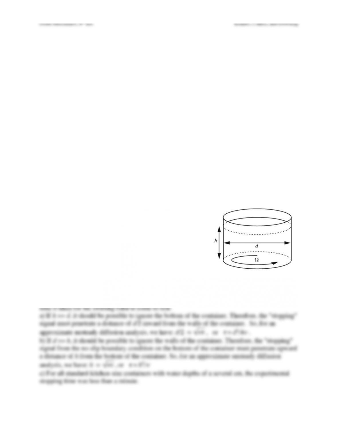
Exercise 10.30. A simple realization of a temporal boundary layer involves the spinning fluid in
a cylindrical container. Consider a viscous incompressible fluid (density =
ρ
, viscosity = µ) in
solid body rotation (rotational speed = Ω) in a cylindrical container of diameter d. The mean
depth of the fluid is h. An external stirring mechanism forces the fluid to maintain solid body
rotation. At t = 0, the external stirring ceases. Denote the time for the fluid to spin-down (e.g. to
stop rotating) by
τ
.
a) Case I: h >> d. Write a simple laminar-flow scaling law for
τ
assuming that the velocity
perturbation produced by the no-slip condition on the container’s sidewall must travel inward a
distance d/2 via diffusion.
b) Case II: h << d. Write a simple laminar-flow scaling law for
τ
assuming that the velocity
perturbation produced by the no-slip condition on the container’s bottom must travel upward a
distance h via diffusion.
c) Using partially-filled cylindrical containers of several different sizes (drinking glasses and
pots & pans are suggested) with different amounts of water, test the validity of the above
diffusion estimates. Use a spoon or a whirling motion of the container to bring the water into
something approaching solid body rotation. You’ll know when you’re close to solid body rotation
because the fluid surface will be a paraboloid of revolution. Once you have this initial flow
condition set-up, cease the stirring or whirling and note how long it takes for the fluid to stop
moving. Perform at least one test when d & h are several inches or more. Cookie or bread
crumbs sprinkled on the water surface will help visualize surface motion. The judicious addition
of a few drops of milk after the fluid starts slowing down may prove interesting.
d) Compute numbers from your scaling laws for parts a) and
b) using the viscosity of water, the dimensions of the
containers, and the experimental water depths. Are the scaling
laws from parts a) and b) useful for predicting the
experimental results? If not, explain why.
(The phenomena investigated here have some important
practical consequences in atmospheric and oceanic flows and
in IC engines where swirl and tumble are exploited to mix the
fuel charge and increase combustion speeds.)
Solution 10.30. For all simple unsteady diffusion problems, the length scale of “diffusion-
penetration” is proportional to the square root of the product of the diffusion constant and time.
For momentum diffusion in fluid flows,
ν
is the diffusion constant. In the following, let
τ
be the
time it takes for the swirling fluid to come to rest.
Fluid Mechanics, 6th Ed. Kundu, Cohen, and Dowling
Fluid Mechanics, 6th Ed. Kundu, Cohen, and Dowling
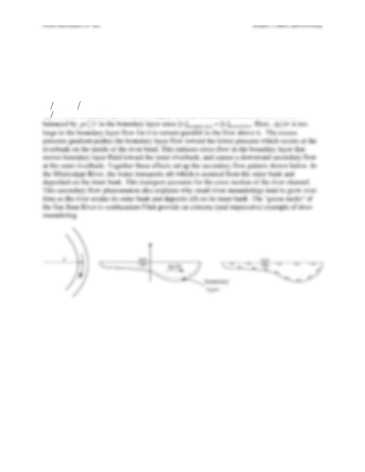
Exercise 10.31. Mississippi River boatmen know that when rounding a bend in the river, they
must stay close to the outer bank or else they will run aground. Explain in fluid mechanical terms
the reason for the cross-sectional shape of the river at the bend.
Solution 10.31. The Reynolds number based on mean channel width or radius of curvature is
very large. Thus, the riverbed boundary layer is thin compared with the width or depth of the
river, and most of the flow is inviscid. The primary turning flow around the bend is governed by
∂
p
∂
r=
ρ
v
θ
2r
, but v
θ
decreases rapidly to zero in the thin boundary layer on the riverbed. Thus,
∂
p
∂
r
in the boundary layer, which is largely the same as that in the inviscid flow, is not
balanced by
ρ
v
θ
2r
in the boundary layer since [v
θ
]boundary layer < [v
θ
]inviscid flow. Here,
∂
p
∂
r
is too