Fluid Mechanics, 6th Ed. Kundu, Cohen, and Dowling
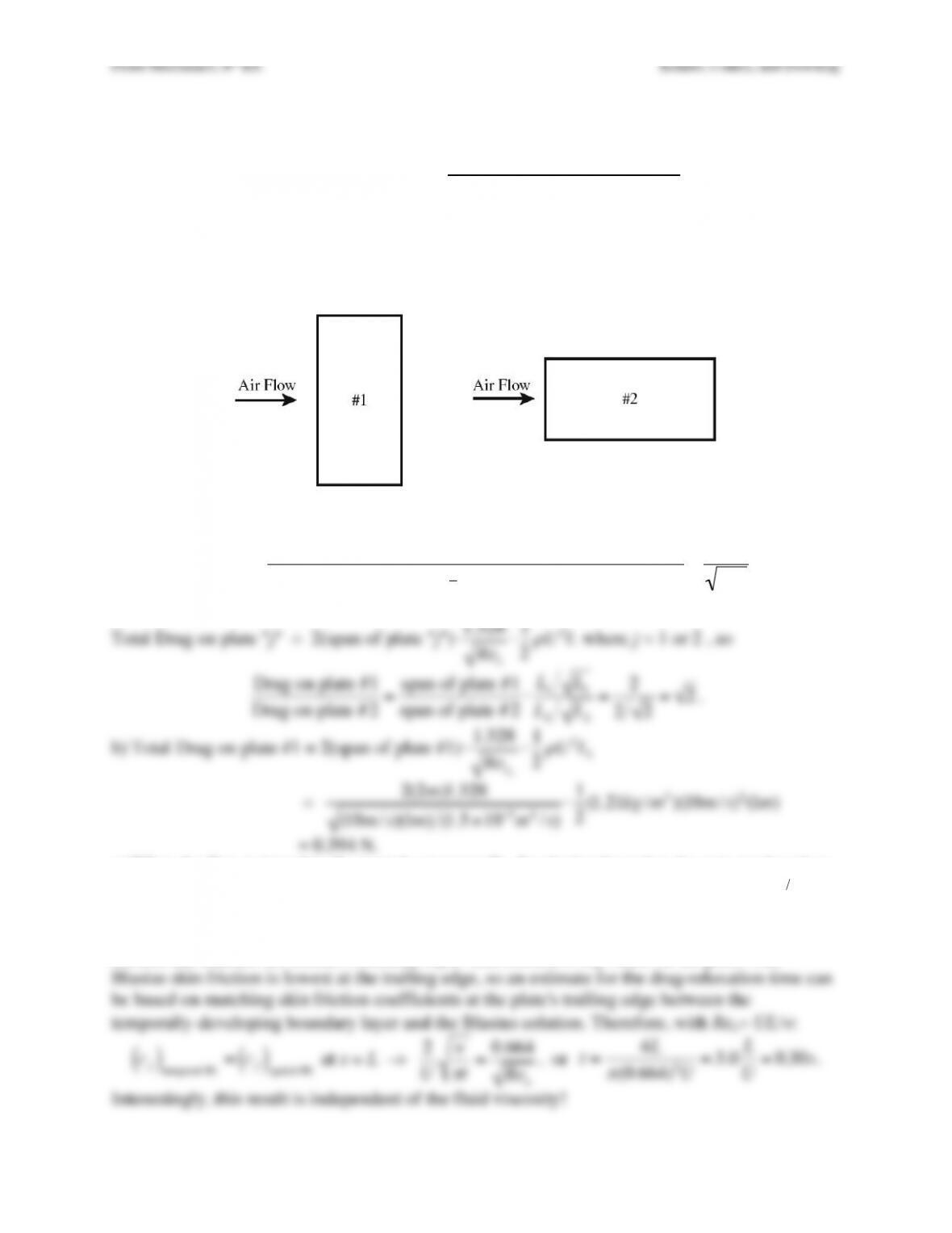
Exercise 10.1. A thin flat plate 2 meters long and 1 meter wide is placed at zero angle of attack
in a low speed wind tunnel in the two positions sketched below.
a) For steady airflow, what is the ratio: drag on the plate in position #1
drag on the plate in position #2 ?
b) For steady airflow at 10 m/sec, what is the total drag on the plate in position #1?
c) If the air flow is impulsively raised from zero to 10 m/sec at t = 0, will the initial drag on the
plate in position #1 be greater or less than the steady-state drag value calculated for part b)?
d) Estimate how long it will take for drag on the plate in position #1 in the impulsively started
flow to reach the steady-state drag value calculated for part b)?
Solution 10.1. a) Here we need only consider the drag coefficient, CD, from the Blasius solution.
CD(L)=Drag per unit span on one side of the plate of length L
( )
1
2
ρ
U2L=1.328
ReL
where ReL= UL/
ν
. Therefore:
Total Drag on plate “j” = 2(span of plate “j“)
⋅1.328
⋅1
2
ρ
U2L
where j = 1 or 2 , so
the top and bottom of plate #1. Initially, the shear stress is very high since:
τ
w≅
µ
U(
πν
t)−1 2
so
the initial drag will be greater than the steady-state drag.
d) The flow will have reached steady-state when the temporally developing boundary layer skin
friction has reached the Blasius boundary layer skin friction everywhere on the plate. The
Blasius skin friction is lowest at the trailing edge, so an estimate for the drag-relaxation time can
Fluid Mechanics, 6th Ed. Kundu, Cohen, and Dowling
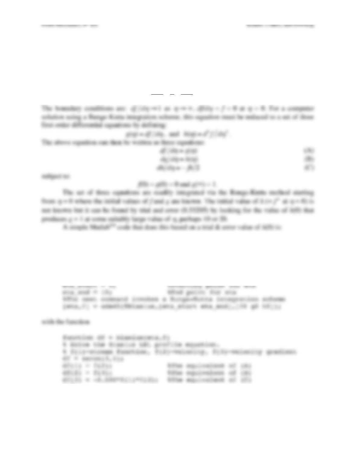
Exercise 10.2. Solve the Blasius equations (10.27) through (10.29) with a computer, using the
Runge–Kutta scheme of numerical integration, and plot the results. What value of
!!
f
at
η
= 0
leads to a successful profile?
Solution 10.2. The Blasius equation is a non-linear third-order differential equation for f(
η
):
d3f
d
η
3+1
2fd2f
d
η
2=0
.
The boundary conditions are:
df d
η
→1
as
η
→ ∞
, df/d
η
= f = 0 at
η
= 0. For a computer
!!
f
%Compute the Blasius Boundary Layer Profile
clear;
clc;
f0 = 0; %The first known boundary condition
g0 = 0; %The second known boundary condition
h0 = 0.33205; %The value adjusted by trial & error
eta_start = 0; %Starting point for eta
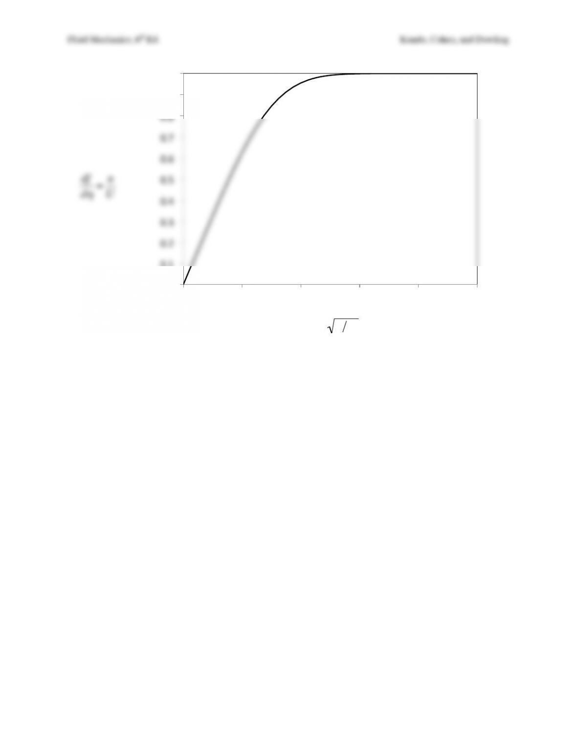
The resulting plot of df/d
η
vs.
η
is:
Fluid Mechanics, 6th Ed. Kundu, Cohen, and Dowling
!”
!#$”
!#%”
!#&”
!#'”
!#(“
!#)”
!#*”
!#+”
!#,”
$”
!” %” ‘” )” +” $!”
df
d
η
=u
U
η
=y U
ν
x
Fluid Mechanics, 6th Ed. Kundu, Cohen, and Dowling
Exercise 10.3. A flat plate 4 m wide and 1 m long (in the direction of flow) is immersed in
kerosene at 20°C, (v = 2.29 × 10⁻⁶ m2/s,
ρ
= 800 kg/m3) flowing with an undisturbed velocity of
0.5 m/s. Verify that the Reynolds number is less than critical everywhere, so that the flow is
laminar. Show that the thickness of the boundary layer and the shear stress at the center of the
plate are
δ
= 0.74 cm and τ0 = 0.2 N/m2, and those at the trailing edge are
δ
= 1.05 cm and τ0 =
0.14 N/m2. Show also that the total frictional drag on one side of the plate is 1.14 N. Assume that
the similarity solution holds for the entire plate.
Solution 10.3. ReL = UL/
ν
= (0.5m/s)(1m)/(2.29×106 m2/s) = 2.18×10⁵ < Recr ~ 106. Thus, the
flow is expected to be laminar everywhere.
At x = 0.5 m, Rex = 1.09×10⁵ so the 99% thickness from (10.30) and the shear stress from (10.31)
are:
δ
99 =4.9xRex
1 2 =4.9(0.5) 1.09 ×105=0.742cm
, and
τ
0=0.332
ρ
U2Rex
1 2 =0.332(800)(0.5)21.09 ×105=0.201N/m2
.
At x = 1.0 m, Rex = 2.18×10⁵ so
δ
99 =4.9xRex
1 2 =4.9(1.0) 2.18 ×105=1.05cm
, and
τ
0=0.332
ρ
U2Rex
1 2 =0.332(800)(0.5)22.18 ×105=0.142N/m2
.
The total drag can be obtained from (10.33):
CD=1.33 Rex
1 2 =2.85 ×10⁻³
, so
D=1
2
ρ
U2(Area)CD=0.5(800)(0.5)2(4)(1)(0.00285) =1.14N
.
Fluid Mechanics, 6th Ed. Kundu, Cohen, and Dowling
Exercise 10.4. A fluid with constant density and viscosity flows with a constant horizontal speed
U∞ over an infinite flat porous plate placed at y = 0 through which fluid is drawn with a constant
velocity Vs. For this flow the steady two-dimensional zero-pressure-gradient boundary layer
equations are (7.2) and (10.18) and the boundary conditions are u(y = 0) = 0, v(y = 0) = –Vs, and
u = U∞ for
y→ ∞
.
a) Assuming u depends only on y, determine u(y) in terms of
ν
, Vs, U∞, and y.
b) What is the wall shear stress
τ
w? How does it depend on
µ
?
c) What parametric change(s) decrease the boundary layer thickness?
Solution 10.4. a) If u = u(y), then ∂u/∂x = 0 = ∂v/∂y and this means that v is a most a function of
x. However, the boundary condition on v at y = 0 does not depend on x, thus v = const. = –Vs.
Therefore, the horizontal momentum equation simplifies to:
−Vs
∂
u
∂
y=
ν∂
2u
∂
y2
, which can be
Fluid Mechanics, 6th Ed. Kundu, Cohen, and Dowling
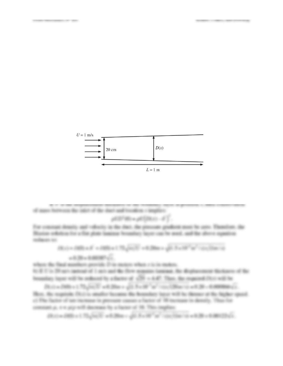
Exercise 10.5. A square-duct wind tunnel test section of length L = 1 m is being designed to
operate at room temperature and atmospheric conditions. A uniform air flow at U = 1 m/s enters
through an opening of D = 20 cm. Due to the viscosity of air, it is necessary to design a variable
cross-sectional area if a constant velocity is to be maintained in the middle part of the cross-
section throughout the wind tunnel.
a) Determine the duct size, D(x), as a function of x.
b) How will the result be affected if U = 20 m/s? At a given value of x, will D(x) be larger or
smaller than (or the same as) the value obtained in a)? Explain.
c) How will the result be affected if the wind tunnel is to be operated at 10 atm (and U = 1 m/s)?
At a given value of x, will D(x) be larger or smaller than (or the same as) the value obtained in
a)? Explain. [Hint: the dynamic viscosity of air (
µ
[N·s/m2]) is largely unaffected by pressure.]
d) Does the airflow apply a net force to the wind tunnel test section? If so, indicate the direction
of the force.
Solution 10.5. a) The duct length (1 m) and the flow speed (1 m/s) imply a Reynolds number of:
ReL = UL/
ν
= (1 m/s)(1 m)/(1.5×10–5m2/s) = 67,000, which much larger than unity but still in the
laminar boundary layer range.
If
δ
* is the displacement thickness of the boundary layer at position x, then conservation
Fluid Mechanics, 6th Ed. Kundu, Cohen, and Dowling
So, the requisite D(x) will be smaller than the part a) result because the boundary layer will be
Fluid Mechanics, 6th Ed. Kundu, Cohen, and Dowling
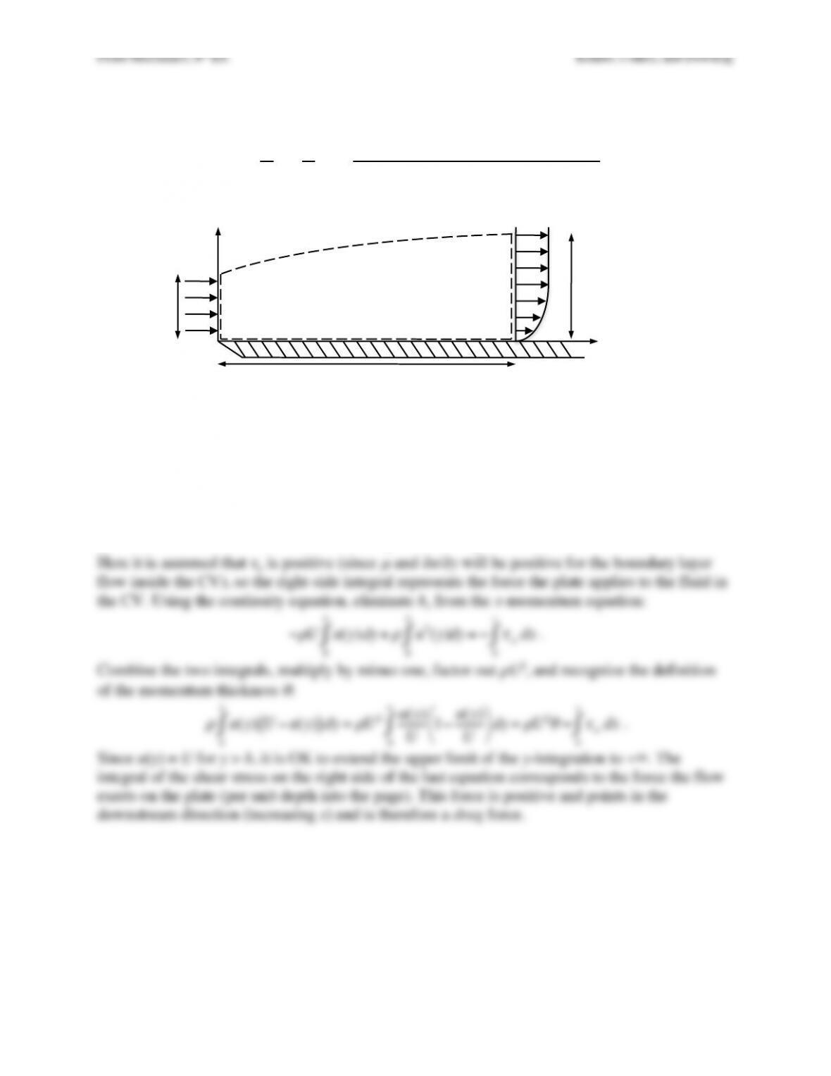
Exercise 10.6. Use the control volume shown to derive the definition of the momentum
thickness,
θ
, for flow over a flat plate:
ρ
U2
θ
=
ρ
U2u
U1−u
U
“
#
$%
&
‘
0
h
∫dy =Drag force on the plate from zero to x
unit depth into the page =
τ
wdx
0
x
∫
The words in the figure describe the upper and lower control volume boundaries.
Solution 10.6. The CV is stationary, so the integral form of the continuity equation is:
ρ
Uho=
ρ
u(y)dy
0
h
∫
,
where h is defined in the figure to be greater than the boundary layer thickness. The pressure is
the same everywhere so the integral form of the x-momentum equation is:
−
ρ
U2ho+
ρ
u2(y)
0
h
∫dy =−
τ
wdx
0
x
∫
.
Here it is assumed that
τ
w is positive (since
µ
and ∂u/∂y will be positive for the boundary layer
U!
h >
δ
99!
ho!
U!
zero shear stress, !
constant pressure, no through flow!
y!
x!
no slip,
τ
w ≠ 0!
Fluid Mechanics, 6th Ed. Kundu, Cohen, and Dowling
Exercise 10.7. Estimate the 99% boundary layer thickness on:
a) a paper airplane wing (length = 0.25 m, U = 1 m/sec),
b) the underside of a super tanker (length = 300 m, U = 5 m/sec), and
c) an airport run way on a blustery day (length = 5 km, U = 10 m/sec).
d) Will these estimates be accurate in each case? Explain.
Solution 10.7. Estimate the various thicknesses from the laminar zero-pressure-gradient
(Blasius) boundary layer solution:
δ
99 =4.9
ν
x U
.
a)
δ
99 =4.9 (1.5 ×10⁻⁵m2s–1)(0.25m) (1ms−1)=9.5mm
Fluid Mechanics, 6th Ed. Kundu, Cohen, and Dowling
Exercise 10.8. Air at 20°C and 100 kPa (
ρ
= 1.167 kg/m3,
ν
= 1.5 × 10⁻⁵ m2/s) flows over a thin
plate with a free-stream velocity of 6 m/s. At a point 15 cm from the leading edge, determine the
value of y at which u/U = 0.456. Also calculate v and ∂u/∂y at this point. [Answer: y = 0.857 mm,
v = 0.384 cm/s, ∂u/∂y = 3012 s–1.]
Solution 10.8. From Table 10.1,
η
=y U
ν
x=1.4
when u/U = 0.456. Therefore,
y=1.4
ν
x U =1.4 (1.5×10⁻⁵)(0.15) 6
= 0.857 mm.
At this wall normal distance, the Blasuis BL formula for v and Table 10.1 produce:
v=1
2
ν
U
x−f+
η
df
d
η
“
#
$%
&
‘=1
2
1.5×10⁻⁵(6)
0.15 −0.325 +1.4 ⋅0.456
( )
= 0.00384 m/s.
Again using Table 10.1, the slope of the velocity profile is:
∂
u
∂
y=U
∂
(u/U)
∂η
∂η
∂
y=U!!
f U
ν
x=(6)(0.3074) 6 (1.5×10⁻⁵)(0.15)
= 3012 s–1.
Fluid Mechanics, 6th Ed. Kundu, Cohen, and Dowling
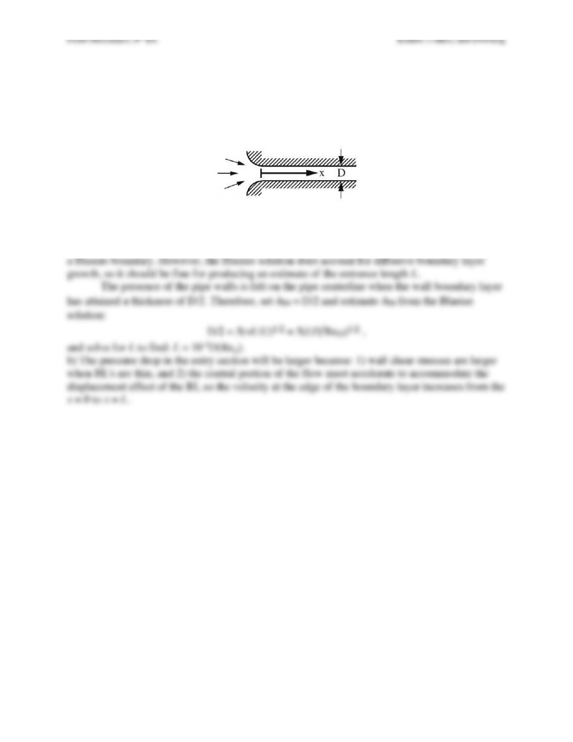
Exercise 10.9. An incompressible fluid (density
ρ
, viscosity µ) flows steadily from a large
reservoir into a long pipe with diameter D. Assume the pipe-wall boundary layer thickness is
zero at x = 0. The Reynolds number based on D, ReD, is greater than 104.
a) Estimate the necessary pipe length for establishing a parabolic velocity profile in the pipe.
b) Will the pressure drop in this entry length be larger or smaller than an equivalent pipe length
in which the flow has a parabolic profile? Why?
Solution 10.9. a) Fortunately, the exercise asks for an estimate. The flow in the entrance length
of a round pipe will accelerate on the pipe’s centerline, and the inner wall of the pipe is curved.
Both of these features will cause the boundary layer growth inside the pipe to differ from that of
a Blasius boundary. However, the Blasius solution does account for diffusive boundary layer
Fluid Mechanics, 6th Ed. Kundu, Cohen, and Dowling
Exercise 10.10. A variety of different dimensionless groups have been used to characterize the
importance of a pressure gradient in boundary layer flows. Develop an expression for each of the
following parameters for the Falkner-Skan boundary layer solutions in terms of the exponent n in
Ue(x) = axn, Rex = Uex/
ν
, integrals involving the profile function
!
f
, and
!!
f(0)
, the profile slope
at y = 0. Here
u(x,y)=Ue(x)!
f y
δ
(x)
( )
=Ue!
f(
η
)
and the wall shear stress
τ
w=
µ∂
u
∂
y
( )
y=0=
µ
Ue
δ
(x)
( )
!!
f(0)
. What value does each parameter take in a Blasius
boundary layer. What value does each parameter achieve at the separation condition?
a)
ν
Ue
2
( )
dUedx
( )
, an inverse Reynolds number
b) (
θ
2/
ν
)(dUe/dx), the Holstein and Bohlen correlation parameter
c)
µρτ
w
3
( )
dp dx
( )
, Patel’s parameter
d)
δ
*
τ
w
( )
dp dx
( )
, Clauser’s parameter
Solution 10.10. a) Here Ue(x) = axn, so
dUedx =nax n−1
; thus
ν
Ue
2
dUe
dx =
ν
Ue
nax n−1
ax n=n
ν
Uex=n
Rex
.
The profile function does not enter here. This parameter is zero for the Blasius boundary layer,
and is –0.0904/Rex at separation.
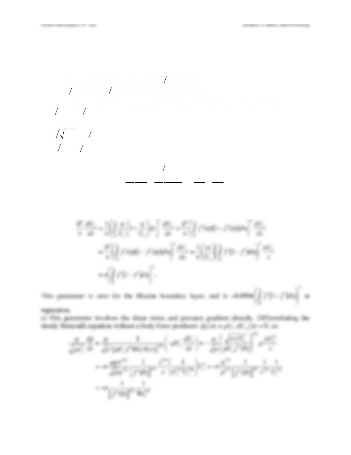
b) This time the profile function enters through the definition of the momentum thickness.
θ
2
ν
dUe
dx =1
ν
u
Ue
1−u
Ue
%
&
‘
(
)
*
0
∞
∫dy
%
&
‘
(
)
*
2
dUe
dx =
δ
2
ν
.
f (
η
) 1−.
f (
η
)
( )
0
∞
∫d
η
%
&
‘ (
)
*
2dUe
dx
=
δ
2
ν
.
f (
η
) 1−.
f (
η
)
( )
0
∞
∫d
η
%
&
‘ (
)
*
2dUe
dx =1
ν
ν
x
Ue
%
&
‘
(
)
* .
f 1−.
f
( )
0
∞
∫d
η
%
&
‘ (
)
*
2nUe
x
=n.
f 1−.
f
( )
0
∞
∫d
η
%
&
‘ (
)
*
2
.
This parameter is zero for the Blasius boundary layer, and is –0.0904
“
f 1−“
f
( )
0
∞
∫d
η
‘
(
) *
+
,
2
at
separation.
c) This parameter involves the shear stress and pressure gradient directly. Differentiating the
steady Bernoulli equation without a body force produces
dp dx +
ρ
UedUedx =0
, so
µ
ρτ
w
3
dp
dx =
µ
ρ
1
µ
Ue!!
f(0)
δ
(x)
( )
3 2 −
ρ
Ue
dUe
dx
#
$
%&
‘
(=−
µ
ρ
ν
x Ue
µ
Ue!!
f(0)
#
$
%
%
&
‘
(
(
3 2
ρ
nUe
2
x
=−n
µρν
3 4
ρµ
3 2
1
!!
f(0)
[ ]
3 2
x3 4
x
1
Ue
3 2Ue
3 4
#
$
%&
‘
(Ue
2=−n
µ
1 4
ρ
1 4
1
!!
f(0)
[ ]
3 2
1
x1 4
1
Ue
1 4
=−n1
!!
f(0)
[ ]
3 2
1
Rex
1 4
Fluid Mechanics, 6th Ed. Kundu, Cohen, and Dowling
Fluid Mechanics, 6th Ed. Kundu, Cohen, and Dowling
Solution 10.11. Consider the boundary layer that develops as a constant density viscous fluid is
drawn to a point sink at x = 0 on and infinite flat plate in two dimensions (x, y). Here Ue(x) = –
UoLo/x, so set
η
=y
ν
x|Ue|
and
ψ
=−
ν
x|Ue|f(
η
)
and redo the steps leading to (10.36) to
find
“ “ “
f −“
f 2+1=0
. Solve this equation and utilize appropriate boundary conditions to find
“
f =31−
α
e−2
η
1+
α
e−2
η
&
‘
(
)
*
+
2
−2
where
α
=3−2
3+2
.
Exercise 10.11. Use the specified Ue to develop the appropriate expressions for
ψ
and h.
ψ
=
ν
x|Ue|f(
η
)=
ν
xUoLo
xf(
η
)=
ν
UoLof(
η
)
, and
η
=y
ν
x|Ue|=y
ν
x2UoLo
=UoLo
ν
y
x
.
The Cartesian velocity components are:
Fluid Mechanics, 6th Ed. Kundu, Cohen, and Dowling
Now set
F=3 tanh(
γ
)
, so that
dF =3 1−tanh2(
γ
)
( )
d
γ
, thus
2dF
3−F2
∫=2 3 1−tanh2(
γ
)
( )
d
γ
3 1−tanh2(
γ
)
( )
∫=2
3
γ
=2
3tanh−1F
3
%
&
‘ (
)
* =2
3
η
+C
Backtracking all the way to
“
f
produces:
2
3
η
+C=2
3
tanh−12+$
f
3
%
&
‘
(
)
*
.
The constant C can be evaluated from
“
f (0) =0
:
C=2
“
tanh−12
3
#
%
&
(
To reach the desired form, use the sum formula for the hyperbolic tangent, and the definition of
the hyperbolic tangent. Then manipulate the exponentials and the square roots.
“
f =3
tanh
η
2
( )
+2 3
1+tanh
η
2
( )
2 3
$
%
&
&
‘
(
)
)
2
−2=3
e
η
2−e−
η
2
e
η
2+e−
η
2+2
3
1+e
η
2−e−
η
2
e
η
2+e−
η
2
+
,
–
.
/
0 2
3
$
%
&
&
&
&
&
‘
(
)
)
)
)
)
2
−2=3
1−e−2
η
1+e−2
η
+2
3
1+1−e−2
η
1+e−2
η
+
,
–
.
/
0 2
3
$
%
&
&
&
&
&
‘
(
)
)
)
)
)
2
−2
=3
1−e−2
η
+2
3
1+e−2
η
( )
1+e−2
η
+1−e−2
η
( )
2
3
$
%
&
&
&
&
‘
(
)
)
)
)
2
−2=3
3−3e−2
η
+2 1+e−2
η
( )
3+3e−2
η
+2 1−e−2
η
( )
$
%
&
&
‘
(
)
)
2
−2
=3
3+2−3−2
( )
e−2
η
3+2+3−2
( )
e−2
η
$
%
&
&
‘
(
)
)
2
−2=3
1−3−2
3+2
+
,
–
.
/
0
e−2
η
1+3−2
3+2
+
,
–
.
/
0
e−2
η
$
%
&
&
&
&
&
‘
(
)
)
)
)
)
2
−2.
The final equality is the desired form.
Fluid Mechanics, 6th Ed. Kundu, Cohen, and Dowling
Exercise 10.12. Start from the boundary layer equations, (7.2), (10.9), and (10.10), and
ψ
=Ue(x)
δ
(x)f(
η
)
, where
η
=y
δ
(x)
, with
δ
(x) unspecified, to complete the following items.
a) Show that the boundary-layer profile equation can be written:
!!!
f+
α
f!!
f+
β
(1−!
f2)=0
, where
α
=
δ ν
( )
d(Ue
δ
)dx
, and
β
=
δ
2
ν
( )
dUedx
.
b) The part a) equation will yield similarity solutions when
α
and
β
do not depend on x.
Therefore, assume
α
and
β
are constants, set Ue = axn, and show that n =
β
/(2
α
–
β
).
c) Deduce the values of
α
and
β
that allow the profile equation to simplify to the Falkner-Skan
profile equation (10.36).
Solution 10.12. a) The given stream function automatically satisfies the continuity equation, so
the next step is to substitute it into (10.9):
u∂u
∂x+v∂u
∂y=Ue
dUe
dx +
ν
∂2u
∂y2
.
Here, the surface-normal boundary-layer momentum equation (10.10), –∂p/∂y = 0, and the
( )
Fluid Mechanics, 6th Ed. Kundu, Cohen, and Dowling
b) When
α
and
β
are constants, their defining equations may be used to eliminate
δ
. Start with
the
α
-equation:
α
=
δ
ν
d(Ue
δ
)
dx =
δ
Ue
ν
d
δ
dx +
δ
2
ν
dUe
dx =Ue
2
ν
d
δ
2
dx +
β
.
Using the two ends of this extended equality, substitute for
δ
2 from the definition of
β
to find a
non-linear equation for Ue:
α
=Ue
2
ν
d
δ
2
dx +
β
=Ue
2
ν
d
dx
νβ
dUedx
!
“
#$
%
&+
β
=−Ue
2
β
dUedx
( )
2
d2Ue
dx2+
β
.
Again using the two ends of this extended equality and simplifying leads to:
α
−
β
β
dUe
dx
“
#
$%
&
‘
2
=−Ue
2
d2Ue
dx2
,
and this equation has power-law solutions: Ue = axn. Substituting this trial solution into this
equation produces:
α
−
β
β
a2n2x2n−2=−axn
2
an(n−1)xn−2
which simplifies to:
α
−
β
β
n=−1
2(n−1)
.
Solving this final algebraic equation for n produces the desired relationship: n =
β
/(2
α
–
β
).
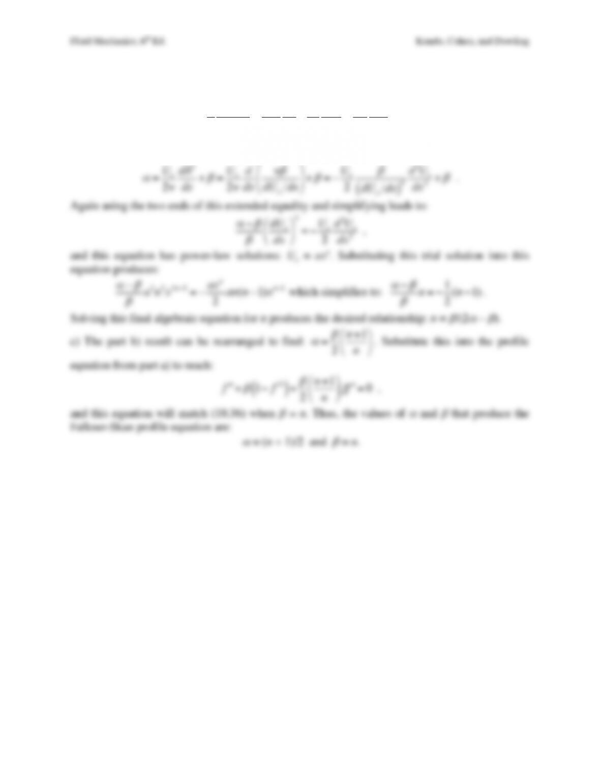
c) The part b) result can be rearranged to find:
α
=
β
2
n+1
n
!
“
#$
%
&
. Substitute this into the profile
equation from part a) to reach:
!!!
f+
β
1−!
f2
( )
+
β
2
n+1
n
#
$
%&
‘
(f!!
f=0
,
and this equation will match (10.36) when
β
= n. Thus, the values of
α
and
β
that produce the
Falkner-Skan profile equation are:
α
= (n + 1)/2 and
β
= n.
Fluid Mechanics, 6th Ed. Kundu, Cohen, and Dowling
Exercise 10.13. Solve the Falkner-Skan profile equation (10.36) numerically for n = –0.0904, –
0.654, 0, 1/9, 1/3, and 1 using boundary conditions (10.28) and (10.29) and the Runge–Kutta
scheme of numerical integration. Plot the results and compare to Figure 10.8. What values of
!!
f
at
η
= 0 lead to successful profiles at these six values of n?
Solution 10.13. The Falkner-Skan profile equation is a non-linear third-order differential
equation for f(
η
):
d3f
d
η
3+n+1
2fd2f
d
η
2−ndf
d
η
“
#
$%
&
‘
2
+n=0
.
The boundary conditions are:
df d
η
→1
as
η
→ ∞
, df/d
η
= f = 0 at
η
= 0. For a computer
solution using a Runge-Kutta integration scheme, this equation must be reduced to a set of three
first-order differential equations by defining:
f1(
η
)=f(
η
)
,
f2(
η
)=df d
η
, and
f3(
η
)=d2f d
η
2
.
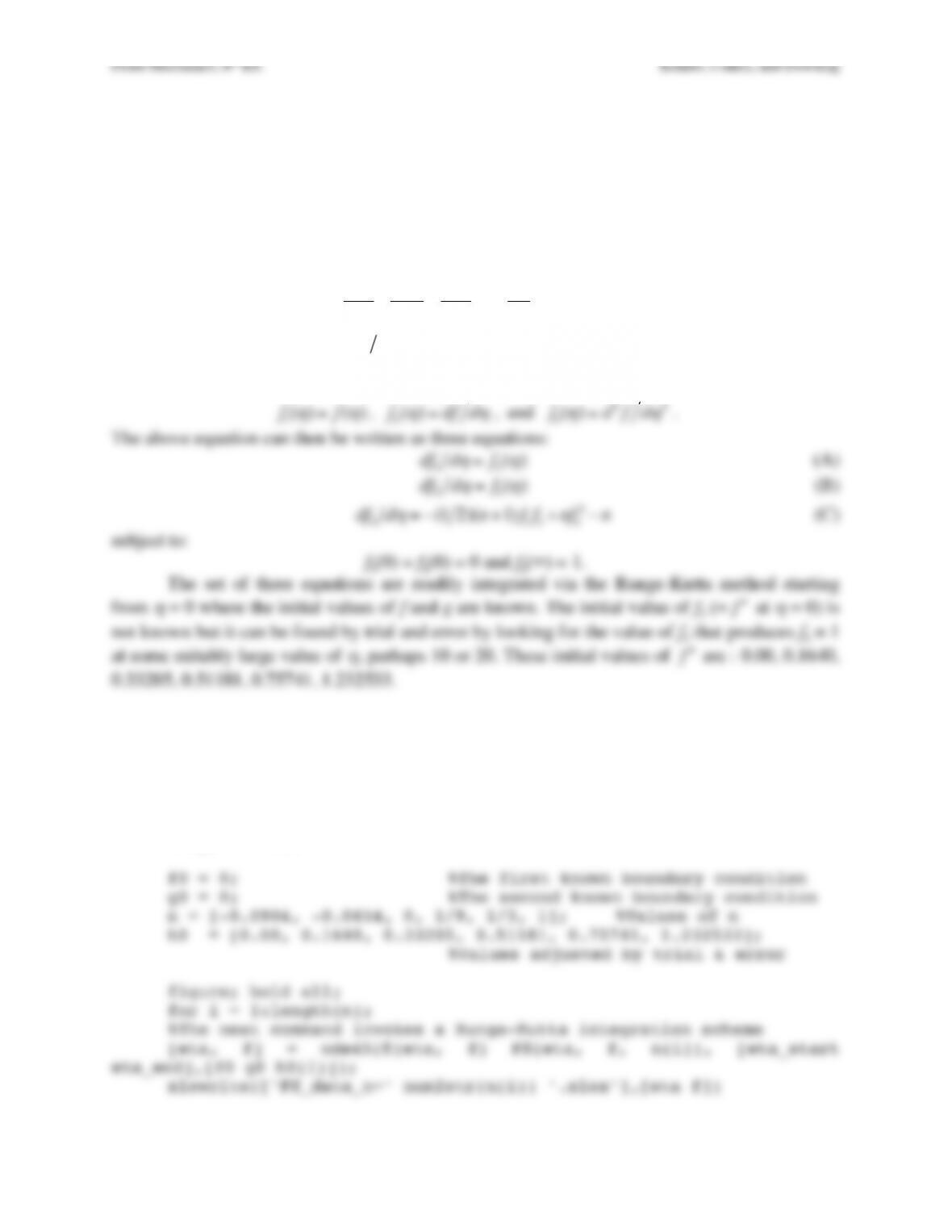
The above equation can then be written as three equations:
df1d
η
=f2(
η
)
(A)
df2d
η
=f3(
η
)
(B)
df3d
η
=−(1 2)(n+1) f1f3+nf2
2−n
(C)
subject to:
f1(0) = f2(0) = 0 and f2(∞) = 1.
The set of three equations are readily integrated via the Runge-Kutta method starting
from
η
= 0 where the initial values of f and g are known. The initial value of f3 (=
!!
f
at
η
= 0) is
A simple MatlabTM code that does this based on a trial & error value of h(0) is:
%Compute the Falkner–Skan Boundary Layer Profile
clear;
clc;
eta_start = 0;
eta_end = 10;
Fluid Mechanics, 6th Ed. Kundu, Cohen, and Dowling
x=(.5*(n(i)+1)).^.5*eta;
plot(x,f(:,2));
end
with the function
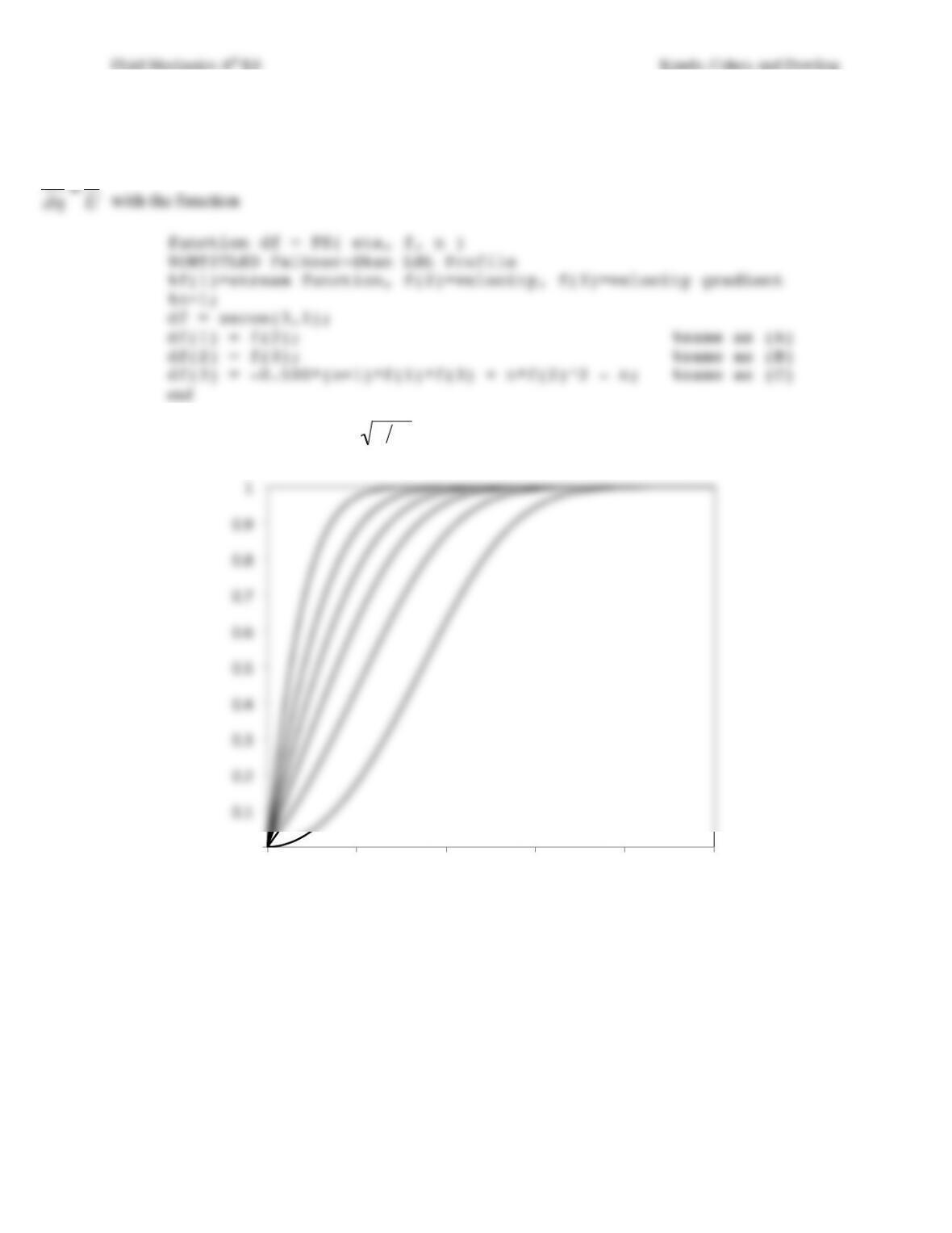
The resulting plot of df/d
η
vs.
η
is:
The left most curve corresponds to n = 1, and the right-most curve corresponds to n = –0.0904
with the other monotonically arrayed in between. And – except for the aspect ratio and extent of
the horizontal axis – this plot is identical to Figure 10.8.
0″
0.1″
0.2″
0.3″
0.4″
0.5″
0.6″
0.7″
0.8″
0.9″
1″
0″ 2″ 4″ 6″ 8″ 10″
df
d
η
=u
U
η
=y U
ν
x
Fluid Mechanics, 6th Ed. Kundu, Cohen, and Dowling
Exercise 10.14. By completing the steps below, show that it is possible to derive von Karman’s
boundary layer integral equation without integrating to infinity in the surface-normal direction
using the three boundary layer thicknesses commonly defined for laminar and turbulent
boundary layers: i)
δ
(or
δ
99) = the full boundary layer thickness that encompasses all (or 99%) of
the region of viscous influence, ii)
δ
* = the displacement thickness of the boundary layer, and iii)
θ
= momentum thickness of the boundary layer. Here, the definitions of the later two involve the
first:
δ
*(x)=1−u(x,y)
Ue(x)
$
%
&
‘
(
)
y=0
y=
δ
∫dy
and
θ
(x)=u(x,y)
Ue(x)1−u(x,y)
Ue(x)
$
%
&
‘
(
)
y=0
y=
δ
∫dy
, where Ue(x) is the flow
speed parallel to the wall outside the boundary layer, and
δ
is presumed to depend on x too.
a) Integrate the two-dimensional continuity equation from y = 0 to
δ
to show that the vertical
velocity at the edge of the boundary layer is:
v(x,y=
δ
)=d
dx Ue(x)
δ
*(x)
( )
−
δ
dUe
dx
.
b) Integrate the steady two-dimensional x-direction boundary layer momentum equation from y =
0 to
δ
to show that:
τ
0
ρ
=d
dx
Ue
2(x)
θ
(x)
( )
+
δ
*(x)
2
dUe
2(x)
dx
.
[Hint: Use Leibnitz’s rule
d
dx f(x,y)dy
a(x)
b(x)
∫=f(x,b)db
dx
#
$
%
&
‘
(
−f(x,a)da
dx
#
$
%
&
‘
( +
∂
f(x,y)
∂
xdy
a(x)
b(x)
∫
to handle
the fact that
δ
=
δ
(x)]
Solution 10.14. Start with
∂
u
∂
x+
∂
v
∂
y=0
, and integrate from y = 0 to
δ
to get:
∂
u
∂
xdy +
0
δ
∫v(x,y=
δ
)=0
where v(x,y=0) = 0. Use Leibnitz’s rule to get the differentiation outside the integral: