
CHAPTER 6.
6.1 Let
1
=
2
=
3
=
be the total risk common to every asset. For an equally weighted
portfolio:
P
22
i
3
1i
2
i
2
P;)
9
1
(3w
=
3
1
The fraction of asset i s’ risk that it contributes to a portfolio is given by
iP
.
Without loss of generality consider asset 1.
P1
=
P1
3
1i ii1 )rw,rcov(
=
P1
3
1i i1i )r,rcov(w
=
P1
11 )r,rcov(
3
1
(since cov
)r,r( ji
= 0 if i
j)
=
3
1
3
12
=
3
1
3
1
0.57735
(check:
)
3
1
)
3
1
(
3
1
w)( 3
1i
3
1i ii
P
iP
Thus, the fraction 0.57735 of the asset’s risk is contributed to the portfolio and the
6.2 This problem ‘starkly’ illustrates the gains to diversification. There are two ways to
solve it.
a. Method 1 : use the hint
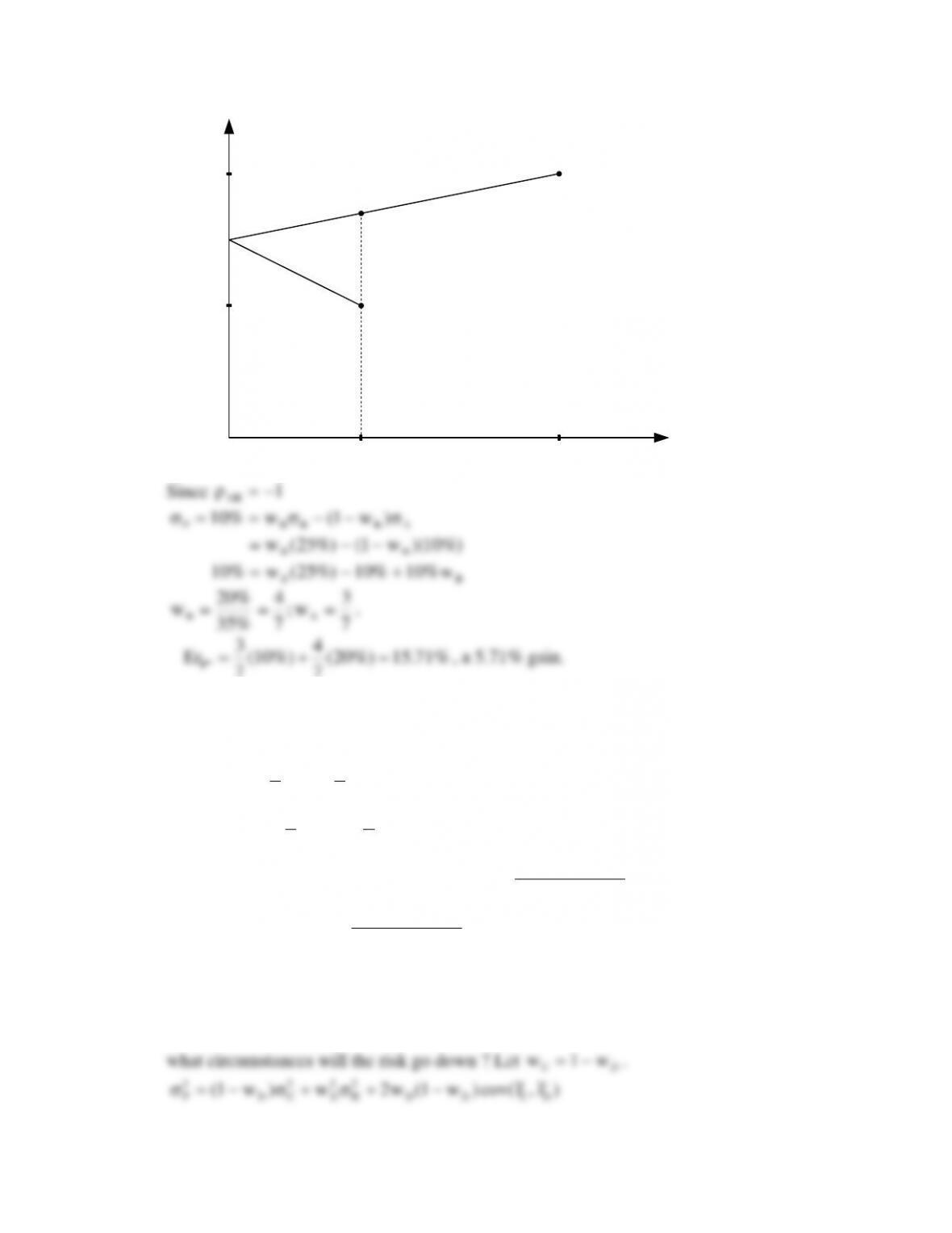
20
10
10 25
A
BP*
7
7
b. Method 2 : first solve for the minimum risk portfolio.
BAAAP )w1(w0
%)25)(w1(%)10(w0 AA
AB
52
w ;w
77
.
%85.12%)20(
7
2
%)10(
7
5
Er
)0
P
(portfoliorisk min
Slope of line joining B + min risk portfolio is
%25
%85.12%20
Thus,
%71.15%)10(
%25
%85.12%20
%85.12Er *P
, a 5.71% gain.
6.3. a. The basis for answering this question is the following :
Let C, D be two assets with
DC
. Let us consider adding some of ‘D’ to ‘C’. Under

Then
D
22
Pw 0 C D C
D
2 cov(r ,r )
w
%%
If
0)r
~
,r
~
cov( 2
CDC
, if we add ‘D’ to ‘C’ the portfolio’s risk will decline below that of
C
.
Equivalently
2
CDC )r
~
,r
~
cov(
2
CDCCD
, or
D
C
CD
or, for the case at hand,
index Aust.
port. your
index Australian port, your
.
b. and c.
So we have to compute these data from the sample statistics that we are given.
24.54.06.24.06.24.54.
6
1
rE
ˆyour
2833.80.20.60.10.10.50.
6
1
rE
ˆ.Aus
22
22222
your
)24.54(.)24.06.(
)24.24(.)24.06.()24.24(.)24.54(.
5
1
ˆ
072.09.09.09.09.
5
1
22
22222 .Aus
)2833.80(.)2833.20(.
)2833.60(.)2833.10(.)2833.10.()2833.50(.
5
1
ˆ
165672.
82836.
5
1
2670.23358.10030.03360.14692.04696.
5
1
.2833)–.24)(.80–(.54
.2833)–.24)(.20–(-.06.2833)–.24)(.60–(.24.2833)–(.10
)24.06.()2833.10.)(24.24(.)2833.50)(.24.54(.
5
1
)r,rcov( .Ausyour
084.
15501.14499.05499.06501.
5
1
now check the above inequality :
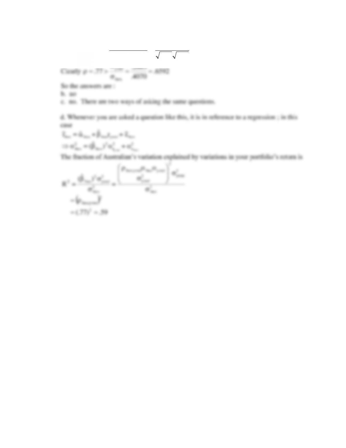
77.
166.072.
084.
)r,rcov(
.Ausyour
.Ausyour
.Aus,your
2683.
your