Intermediate Financial Theory
Danthine and Donaldson
Solutions to Problems
CHAPTER I.
1.1. U is a utility function, i.e., U(x) > U(y) Û x
ℏ
y
then f(U(x)) > f(U(y)) Û U(x) > U(y) Û x
ℏ
y
1.2. Utility function U(
21
c,c
):
FOC: U1/U2=p1/p2
Let f=f(U(.)) be a monotone transformation.
1.3. When an agent has very little of one given good, he is willing to give up a big quantity of
another good to obtain a bit more of the first.
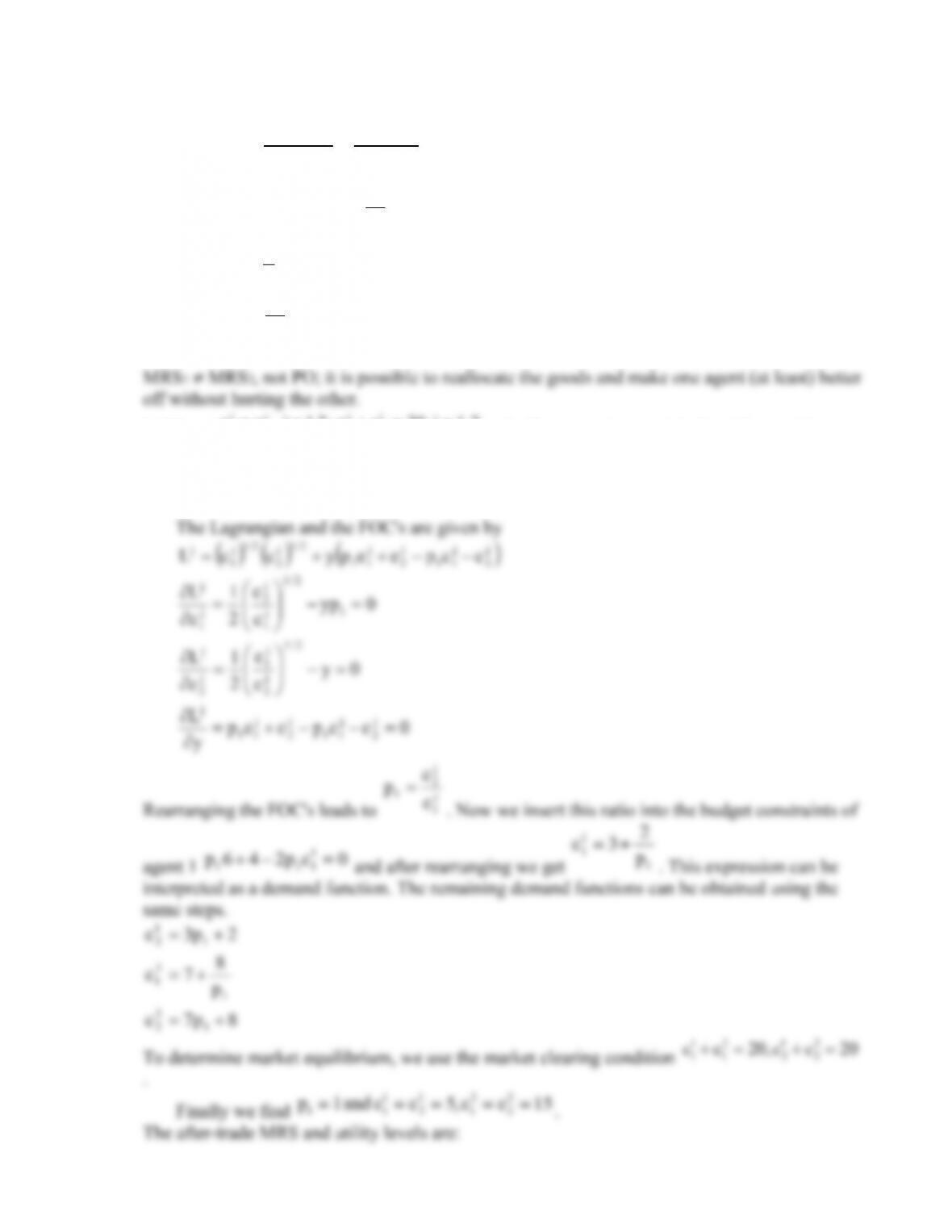
U2 =
5.05.0
1614
= 14.97
j
1
j
2
j
2j
j
1j
j
c1
c
c/U
c/U
MRS
with a = 0.5,
j
1
j
2
j
c
c
MRS
67.0
6
4
MRS
1
14.1
14
16
MRS
2
b) PS = {
1,2i ,20cc :2,1j, cc
i
2
i
1
j
2
j
1
}, the Pareto set is a straight line (diagonal from
lower-left to upper-right corner).
c) The problem of the agents is
j
2
j
11
j
2
j
11
j
ccpeep s.t. MaxU
.
p
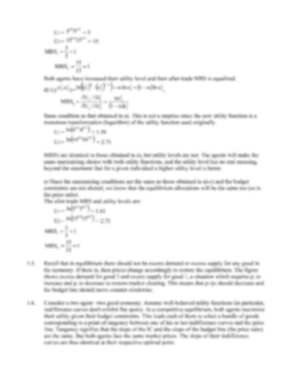
5.05.0
55
1
5
5
MRS
1
1
15
15
MRS
2
Both agents have increased their utility level and their after-trade MRS is equalized.
d) Uj(
j
2
j
1
c,c
) =
j
2
j
1
1
j
2
j
1
cln1clnccln
,
j
1
j
2
j
2j
j
1j
j
c1
c
c/U
c/U
MRS
Same condition as that obtained in a). This is not a surprise since the new utility function is a
monotone transformation (logarithm) of the utility function used originally.
U1 =
5.05.0
46ln
= 1.59
U2 =
5.05.0
1614ln
= 2.71
MRS’s are identical to those obtained in a), but utility levels are not. The agents will make the
same maximizing choice with both utility functions, and the utility level has no real meaning,
beyond the statement that for a given individual a higher utility level is better.
e) Since the maximizing conditions are the same as those obtained in a)-c) and the budget
constraints are not altered, we know that the equilibrium allocations will be the same too (so is
the price ratio).
The after-trade MRS and utility levels are:
U1 =
5.05.0
55ln
= 1.61
U2 =
5.05.0
1515ln
= 2.71
1
5
5
MRS
1
1
15
15
MRS
2
1.5. Recall that in equilibrium there should not be excess demand or excess supply for any good in
the economy. If there is, then prices change accordingly to restore the equilibrium. The figure
1.6. Consider a two agent –two good economy. Assume well-behaved utility functions (in particular,
indifference curves don’t exhibit flat spots). At a competitive equilibrium, both agents maximize
their utility given their budget constraints. This leads each of them to select a bundle of goods
Now consider the second requirement of a competitive equilibrium: that market clear. This
Putting the two elements of this discussion together, we have that a competitive equilibrium is a point
in the box corresponding to a feasible allocation where both agents’ indifference curves are tangent to
Of course, we could have obtained this result simply by invoking the First Welfare Theorem.
1.7. Indifference curves of agent 2 are non-convex.
Point A is a PO : the indifference curves of the two agents are tangent. This PO cannot be obtained as a