Solutions Manual Orbital Mechanics for Engineering Students Third Edition Chapter 5
Howard D. Curtis 191 Copyright © 2013, Elsevier, Inc.
Year = 2007
Month = 12
Day = 21
UT (hr) = 10
West Longitude (deg) = 215.033
East Longitude (deg) = 144.967
Solution:
Local Sidereal Time (deg) = 24.5646
Local Sidereal Time (hr) = 1.63764
—————————————————–
Problem 5.10c: Local sidereal time calculation
Input data:
Year = 2005
Month = 7
Day = 4
UT (hr) = 20
West Longitude (deg) = 118.25
East Longitude (deg) = 241.75
Solution:
Local Sidereal Time (deg) = 104.676
Local Sidereal Time (hr) = 6.9784
–—–—–—–——–—–——–—–——–––—––—––——–—–——
Problem 5.10d: Local sidereal time calculation
Input data:
Year = 2006
Month = 2
Day = 15
UT (hr) = 3
West Longitude (deg) = 43.1
East Longitude (deg) = 316.9
Solution:
Local Sidereal Time (deg) = 146.884
Local Sidereal Time (hr) = 9.79228
–—–—–—–——–—–——–—–——–––—––—––——–—–——
Problem 5.10e: Local sidereal time calculation
Input data:
Year = 2006
Month = 3
Day = 21
UT (hr) = 8
West Longitude (deg) = 228.067
East Longitude (deg) = 131.933
Solution:
Local Sidereal Time (deg) = 70.6348
Local Sidereal Time (hr) = 4.70899

Solutions Manual Orbital Mechanics for Engineering Students Third Edition Chapter 5
–—–—–—–——–—–——–—–——–––—––—–——–—–——–
Solutions Manual Orbital Mechanics for Engineering Students Third Edition Chapter 5
Problem 5.11. Relative to a tracking station whose local sidereal time is 117° and latitude is +51°, the
azimuth and elevation angle of a satellite are 28° and 68°, respectively. Calculate the topocentric right as-
cension and declination of the satellite.
Problem 5.12 A sea-level tracking station at whose local sidereal time is 40 and latitude is 35 makes
the following observations of a space object:
Azimuth: 36.0
Azimuth rate: 0.590
Elevation: 36.6 deg
Elevation rate: –0.263
Range: 988 km
Range rate: 4.86 km/s
What is the state vector of the object?
Solutions Manual Orbital Mechanics for Engineering Students Third Edition Chapter 5
Howard D. Curtis 195 Copyright © 2013, Elsevier, Inc.
% RA = right ascension of the ascending node (rad)
% incl = inclination of the orbit (rad)
% w = argument of perigee (rad)
% TA = true anomaly (rad)
% a = semimajor axis (km)
% rp – perigee radius (km)
% T – period of elliptical orbit (s)
%
% User M-function required: rv_from_observe
% –—–—–——–—–—–—–—–—–—–——–—–——–—–——–––—––—––——–—
clear
global f Re wE mu
deg = pi/180;
f = 0.0033528;
Re = 6378;
wE = 7.2921e-5;
mu = 398600;
%…Data declaration for Problem 5.12:
rho = 988;
rhodot = 4.86;
A = 36;
Adot = 0.59;
a = 36.6;
adot = –0.263;
theta = 40;
phi = 35;
H = 0;
%…
%...Algorithm 5.4:
[r,v] = rv_from_observe(rho, rhodot, A, Adot, a, adot, theta, phi, H);
%...Echo the input data and output the solution to
% the command window:
fprintf(‘–——–—–——––—–—–—–——–—–——–—–——––—––—–‘)
fprintf(‘\n Problem 5.12‘)
fprintf(‘\n\n Input data:\n‘);
fprintf(‘\n Slant range (km) = %g‘, rho);
fprintf(‘\n Slant range rate (km/s) = %g‘, rhodot);
fprintf(‘\n Azimuth (deg) = %g‘, A);
fprintf(‘\n Azimuth rate (deg/s) = %g‘, Adot);
fprintf(‘\n Elevation (deg) = %g‘, a);
fprintf(‘\n Elevation rate (deg/s) = %g’, adot);
fprintf(‘\n Local sidereal time (deg) = %g‘, theta);
fprintf(‘\n Latitude (deg) = %g‘, phi);
fprintf(‘\n Altitude above sea level (km) = %g‘, H);
fprintf(‘\n\n’);
fprintf(‘ Solution:’)
fprintf(‘\n\n State vector:\n’);
fprintf(‘\n r (km) = [%g, %g, %g]’, ...
r(1), r(2), r(3));
fprintf(‘\n v (km/s) = [%g, %g, %g]’, ...
v(1), v(2), v(3));
fprintf(‘\n-—–—–——––—–—–—–——–—–——–—–——––—–—–—-\n’)
Solutions Manual Orbital Mechanics for Engineering Students Third Edition Chapter 5
r3794.7ˆ
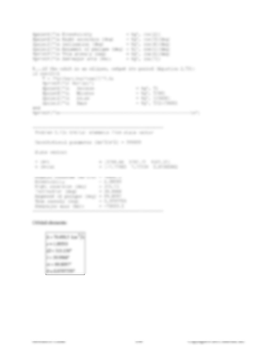
Problem 5.13 Calculate the orbital elements of the satellite in the previous problem.
Solutions Manual Orbital Mechanics for Engineering Students Third Edition Chapter 5
Howard D. Curtis 198 Copyright © 2013, Elsevier, Inc.
fprintf(‘\n Eccentricity = %g’, coe(2))
fprintf(‘\n Right ascension (deg) = %g’, coe(3)/deg)
fprintf(‘\n Inclination (deg) = %g’, coe(4)/deg)
fprintf(‘\n Argument of perigee (deg) = %g‘, coe(5)/deg)
fprintf(‘\n True anomaly (deg) = %g’, coe(6)/deg)
fprintf(‘\n Semimajor axis (km): = %g’, coe(7))
%...if the orbit is an ellipse, output its period (Equation 2.73):
if coe(2)<1
T = 2*pi/sqrt(mu)*coe(7)^1.5;
fprintf(‘\n Period:‘)
fprintf(‘\n Seconds = %g’, T)
fprintf(‘\n Minutes = %g’, T/60)
fprintf(‘\n Hours = %g’, T/3600)
fprintf(‘\n Days = %g’, T/24/3600)
end
fprintf(‘\n—––—–——–—–——–––—––—––——–—–——––—––—––-\n’)
–—–—–—–——–—–——–—–——–––—––—––——–—–——
Problem 5.13: Orbital elements from state vector
Gravitational parameter (km^3/s^2) = 398600
State vector:
r (km) = [3794.66 3792.71 4501.31]
v (km/s) = [–7.72483 7.72134 0.0186586]
i39.9968
89.8097
0.0797759
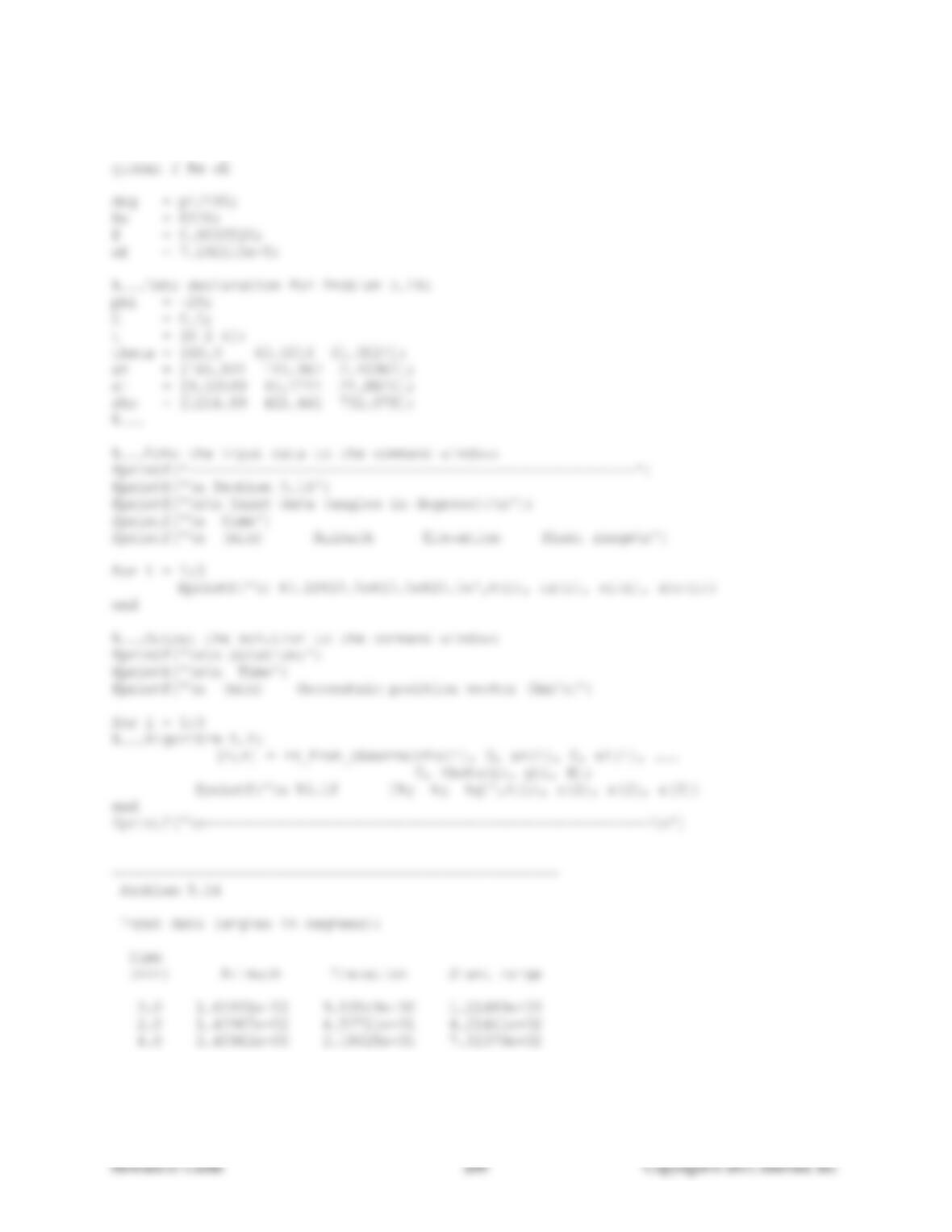
Problem 5.14 A tracking station at latitude –20 and elevation 500 m makes the following observations
of a satellite at the given times.
Time Local sidereal time Azimuth Elevation angle Range
(min) (degrees) (degrees) (degrees) (km)
0 60.0 165.931 9.53549 1214.89
2 60.5014 145.967 45.7711 421.441
4 61.0027 2.40962 21.8825 732.079
Use the Gibbs method to calculate the state vector of the satellite at the central observation time.
Solutions Manual Orbital Mechanics for Engineering Students Third Edition Chapter 5
% –—–—–——–—––—–—–—––—–––—––——–——–—–—–—––——–––——––
clear
Solution:
Time
Howard D. Curtis 201 Copyright © 2013, Elsevier, Inc.
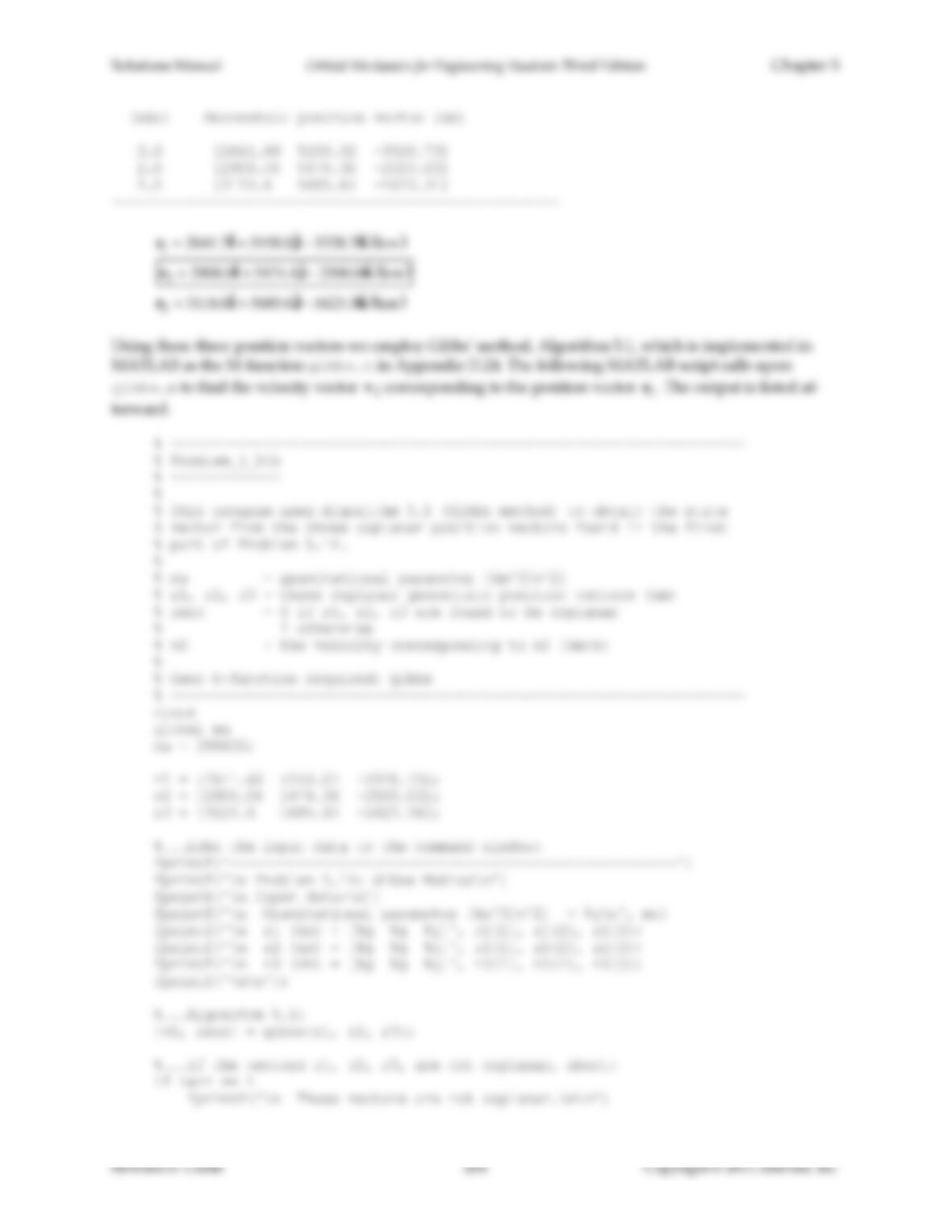
(min) Geocentric position vector (km)
0.0 [2641.68 5158.02 –3328.73]
2.0 [2908.04 5474.36 –2500.03]
4.0 [3118.6 5685.65 –1623.34]
–—–—–—–——–—–——–—–——–––—––—––——–—–——
r
12641.7ˆ
I5158.0ˆ
J3328.7 ˆ
K km
r
22908.0ˆ
I5474.4ˆ
J2500.0 ˆ
K km
r
33118.6ˆ
I5685.6ˆ
J1623.3 ˆ
K km
Using these three position vectors we employ Gibbs’ method, Algorithm 5.1, which is implemented in
MATLAB as the M-function gibbs.m in Appendix D.24. The following MATLAB script calls upon
gibbs.m to find the velocity vector
v2
corresponding to the position vector
r
2
. The output is listed af-
terward.
% ~~~~~~~~~~~~~~~~~~~~~~~~~~~~~~~~~~~~~~~~~~~~~~~~~~~~~~~~~~~~~~~~~~~~
% Problem_5_14b
% ~~~~~~~~~~~~~
%
% This program uses Algorithm 5.1 (Gibbs method) to obtain the state
% vector from the three coplanar position vectors found in the first
% part of Problem 5.14.
%
% mu – gravitational parameter (km^3/s^2)
% r1, r2, r3 – three coplanar geocentric position vectors (km)
% ierr – 0 if r1, r2, r3 are found to be coplanar
% 1 otherwise
% v2 – the velocity corresponding to r2 (km/s)
%
% User M-function required: gibbs
% –—–—–——–—–—–——–—–——–—–—––——–—–——–––—––—––——–—
clear
global mu
mu = 398600;
r1 = [2641.68 5158.02 –3328.73];
r2 = [2908.04 5474.36 –2500.03];
r3 = [3118.6 5685.65 –1623.34];
%...Echo the input data to the command window:
fprintf(‘–——–—–——––—–—–—–——–—–——–—–——––—––—–‘)
fprintf(‘\n Problem 5.14: Gibbs Method\n’)
fprintf(‘\n Input data:\n’)
fprintf(‘\n Gravitational parameter (km^3/s^2) = %g\n‘, mu)
fprintf(‘\n r1 (km) = [%g %g %g]‘, r1(1), r1(2), r1(3))
fprintf(‘\n r2 (km) = [%g %g %g]‘, r2(1), r2(2), r2(3))
fprintf(‘\n r3 (km) = [%g %g %g]‘, r3(1), r3(2), r3(3))
fprintf(‘\n\n’);
%...Algorithm 5.1:
[v2, ierr] = gibbs(r1, r2, r3);
%...If the vectors r1, r2, r3, are not coplanar, abort:
if ierr == 1
fprintf(‘\n These vectors are not coplanar.\n\n’)
Solutions Manual Orbital Mechanics for Engineering Students Third Edition Chapter 5
Howard D. Curtis 202 Copyright © 2013, Elsevier, Inc.
return
end
%...Output the results to the command window:
fprintf(‘ Solution:’)
fprintf(‘\n’);
fprintf(‘\n v2 (km/s) = [%g %g %g]‘, v2(1), v2(2), v2(3))
fprintf(‘\n-—–—–——––—–—–—–——–—–——–—–——––—–—–—-\n’)
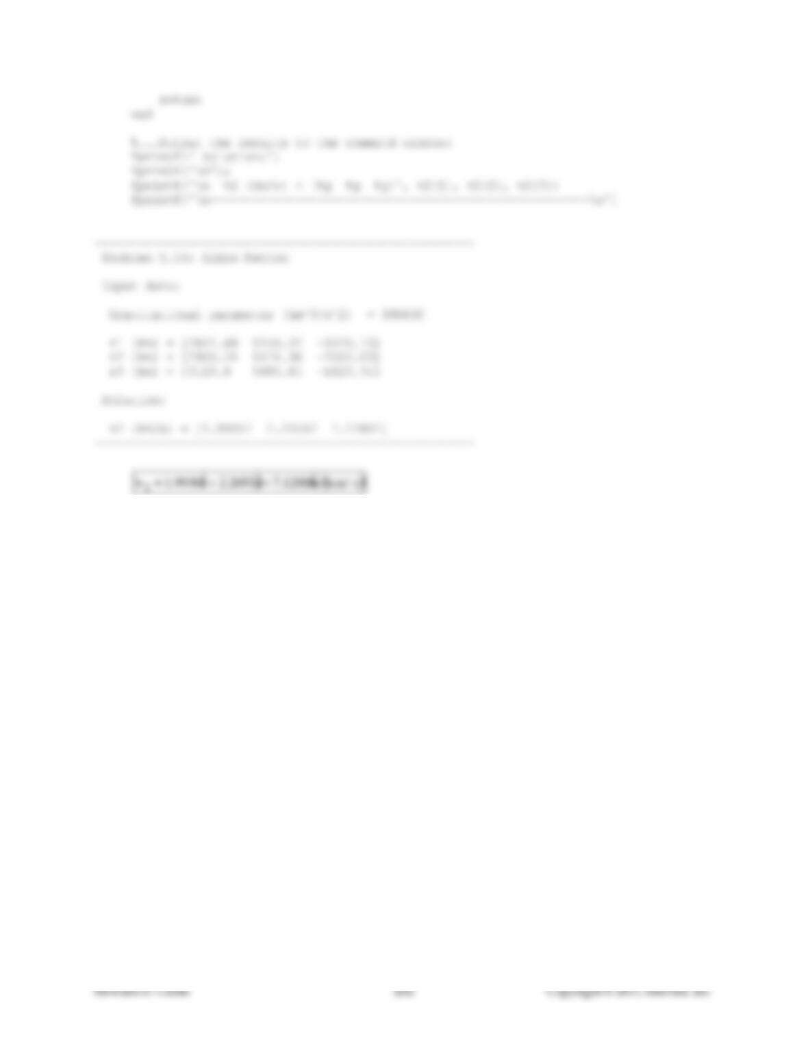
–—–—–—–——–—–——–—–——–––—––—––——–—–——
Problem 5.14: Gibbs Method
Input data:
Gravitational parameter (km^3/s^2) = 398600
r1 (km) = [2641.68 5158.02 -3328.73]
r2 (km) = [2908.04 5474.36 -2500.03]
r3 (km) = [3118.6 5685.65 -1623.34]
Solution:
v2 (km/s) = [1.99357 2.20552 7.12881]
–—–—–—–——–—–——–—–——–——–—–—–——–—–—–
v21.9936ˆ
I2.2055ˆ
J7.1288 ˆ
K km/ s

Problem 5.15 Calculate the orbital elements of the satellite in the previous problem.
% ~~~~~~~~~~~~~~~~~~~~~~~~~~~~~~~~~~~~~~~~~~~~~~~~~~~~~~~~~~~~~~~~~~~~
% Problem_5_15
% ~~~~~~~~~~~~
% –—–—–——–—–—–—–—–—–—–——–—–——–—–——–––—––—––——–—
Solutions Manual Orbital Mechanics for Engineering Students Third Edition Chapter 5
Howard D. Curtis 204 Copyright © 2013, Elsevier, Inc.
fprintf(‘\n Eccentricity = %g’, coe(2))
fprintf(‘\n Right ascension (deg) = %g‘, coe(3)/deg)
fprintf(‘\n Inclination (deg) = %g’, coe(4)/deg)
fprintf(‘\n Argument of perigee (deg) = %g’, coe(5)/deg)
fprintf(‘\n True anomaly (deg) = %g’, coe(6)/deg)
fprintf(‘\n Semimajor axis (km): = %g‘, coe(7))
%...if the orbit is an ellipse, output its period (Equation 2.73):
if coe(2)<1
T = 2*pi/sqrt(mu)*coe(7)^1.5;
fprintf(‘\n Period:‘)
fprintf(‘\n Seconds = %g’, T)
fprintf(‘\n Minutes = %g‘, T/60)
fprintf(‘\n Hours = %g’, T/3600)
fprintf(‘\n Days = %g’, T/24/3600)
end
fprintf(‘\n-—–—–——––—–—–—–——–—–——–—–——––—–—–—-\n’)
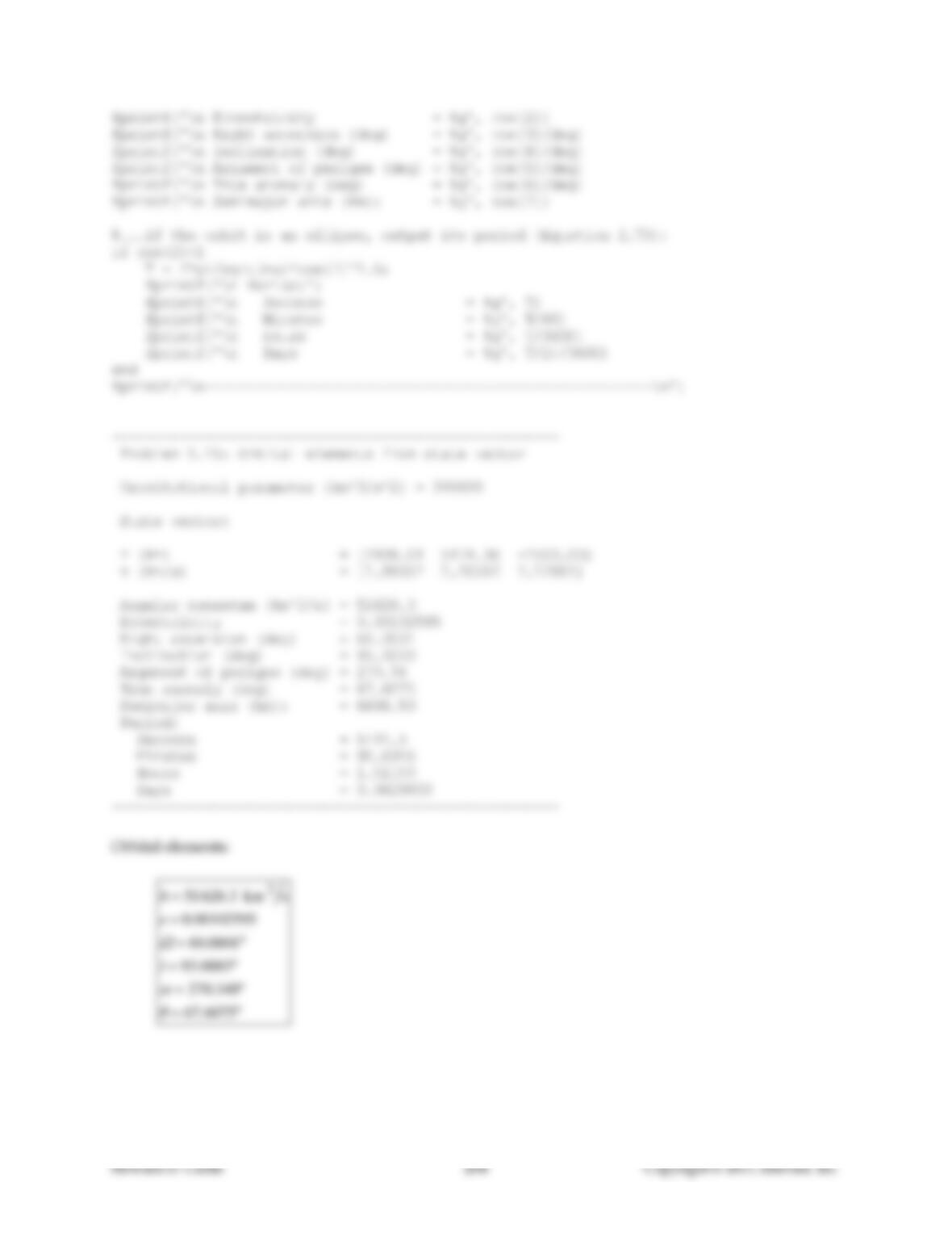
–—–—–—–——–—–——–—–——–––—––—––——–—–——
Problem 5.15: Orbital elements from state vector
Gravitational parameter (km^3/s^2) = 398600
State vector:
r (km) = [2908.04 5474.36 –2500.03]
v (km/s) = [1.99357 2.20552 7.12881]
Angular momentum (km^2/s) = 51626.3
Eccentricity = 0.00102595
Right ascension (deg) = 60.0001
Inclination (deg) = 95.0003
Argument of perigee (deg) = 270.34
True anomaly (deg) = 67.6075
Semimajor axis (km): = 6686.59
Period:
Seconds = 5441.5
Minutes = 90.6916
Hours = 1.51153
Days = 0.0629803
–—–—–—–——–—–——–—–——–––—––—––——–—–——
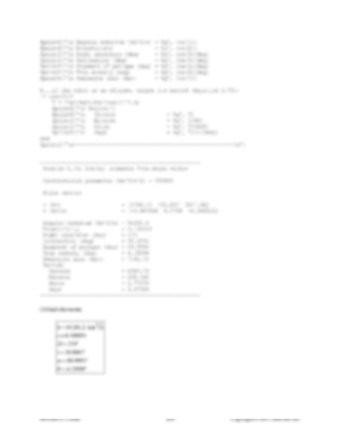
Orbital elements:
h51 626.3 km 2s
e0.00102595
60.0001
i95.0003
270.340
67.6075
Solutions Manual Orbital Mechanics for Engineering Students Third Edition Chapter 5
Problem 5.16 A sea-level tracking station at latitude +29 makes the following observations of a satel-
lite at the given times.
Topocentric Topocentric
Time Local sidereal time Right ascension Declination
(min) (degrees) (degrees) (degrees)
0.0 0 0 51.5110
1.0 0.250684 65.9279 27.9911
2.0 0.501369 79.8500 14.6609
Use the Gauss method without iterative improvement to estimate the state vector of the satellite at the
middle observation time.
Solutions Manual Orbital Mechanics for Engineering Students Third Edition Chapter 5
Howard D. Curtis 206 Copyright © 2013, Elsevier, Inc.
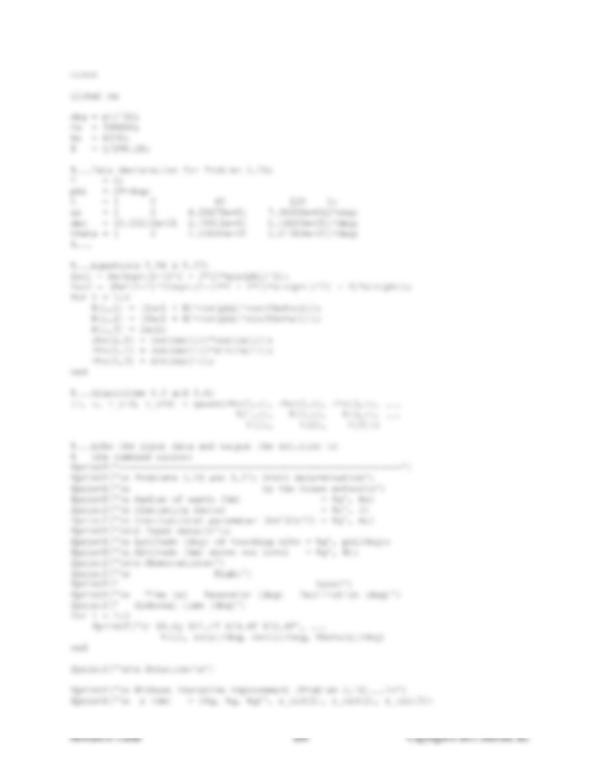
clear
global mu
deg = pi/180;
mu = 398600;
Re = 6378;
f = 1/298.26;
%...Data declaration for Problen 5.16:
H = 0;
phi = 29*deg;
t = [ 0 60 120 ];
ra = [ 0 6.59279e+01 7.98500e+01]*deg;
dec = [5.15110e+01 2.79911e+01 1.46609e+01]*deg;
theta = [ 0 2.50684e–01 5.01369e-01]*deg;
%…
%...Equations 5.56 & 5.57:
fac1 = Re/sqrt(1-(2*f – f*f)*sin(phi)^2);
fac2 = (Re*(1-f)^2/sqrt(1-(2*f – f*f)*sin(phi)^2) + H)*sin(phi);
for i = 1:3
R(i,1) = (fac1 + H)*cos(phi)*cos(theta(i));
R(i,2) = (fac1 + H)*cos(phi)*sin(theta(i));
R(i,3) = fac2;
rho(i,1) = cos(dec(i))*cos(ra(i));
rho(i,2) = cos(dec(i))*sin(ra(i));
rho(i,3) = sin(dec(i));
end
%...Algorithms 5.5 and 5.6:
[r, v, r_old, v_old] = gauss(rho(1,:), rho(2,:), rho(3,:), ...
R(1,:), R(2,:), R(3,:), ...
t(1), t(2), t(3));
%...Echo the input data and output the solution to
% the command window:
fprintf(‘–——–—–——––—–—–—–—–—––—–—–—––—–––——–—‘)
fprintf(‘\n Problems 5.16 and 5.17: Orbit determination‘)
fprintf(‘\n by the Gauss method\n’)
fprintf(‘\n Radius of earth (km) = %g‘, Re)
fprintf(‘\n Flattening factor = %g’, f)
fprintf(‘\n Gravitational parameter (km^3/s^2) = %g‘, mu)
fprintf(‘\n\n Input data:\n‘);
fprintf(‘\n Latitude (deg) of tracking site = %g‘, phi/deg);
fprintf(‘\n Altitude (km) above sea level = %g‘, H);
fprintf(‘\n\n Observations:‘)
fprintf(‘\n Right‘)
fprintf(‘ Local‘)
fprintf(‘\n Time (s) Ascension (deg) Declination (deg)’)
fprintf(‘ Sidereal time (deg)‘)
for i = 1:3
fprintf(‘\n %9.4g %11.4f %19.4f %20.4f‘, ...
t(i), ra(i)/deg, dec(i)/deg, theta(i)/deg)
end
fprintf(‘\n\n Solution:\n’)
fprintf(‘\n Without iterative improvement (Problem 5.16)...\n’)
fprintf(‘\n r (km) = [%g, %g, %g]’, r_old(1), r_old(2), r_old(3))
Solutions Manual Orbital Mechanics for Engineering Students Third Edition Chapter 5
Howard D. Curtis 207 Copyright © 2013, Elsevier, Inc.
fprintf(‘\n v (km/s) = [%g, %g, %g]’, v_old(1), v_old(2), v_old(3))
fprintf(‘\n’);
fprintf(‘\n\n With iterative improvement (Problem 5.17)...\n‘)
fprintf(‘\n r (km) = [%g, %g, %g]’, r(1), r(2), r(3))
fprintf(‘\n v (km/s) = [%g, %g, %g]’, v(1), v(2), v(3))
fprintf(‘\n-—–—–——––—–—–—–——–—–———–—––—–—––—––-\n’)
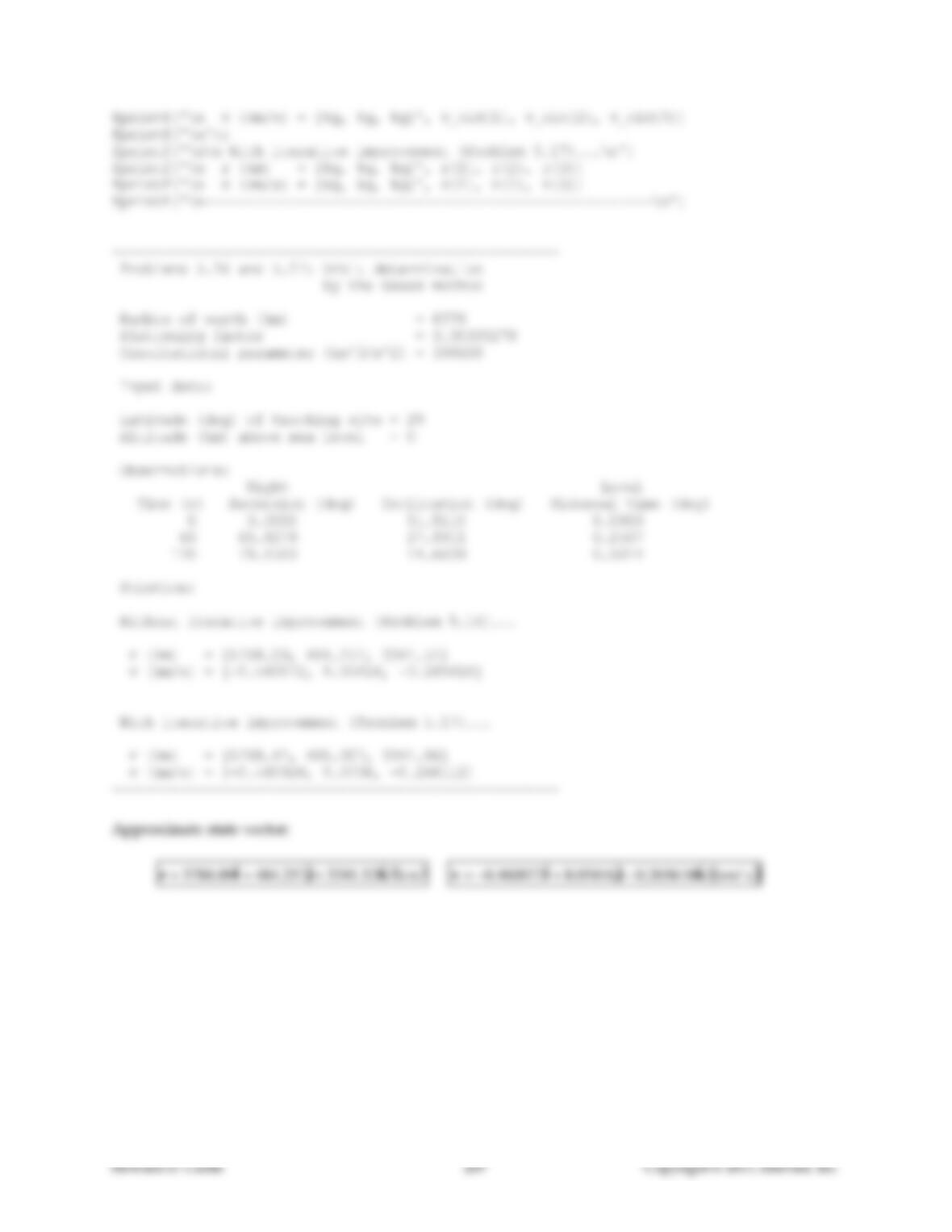
–—–—–—–——–—–——–—–——–––—––—––——–—–——
Problems 5.16 and 5.17: Orbit determination
by the Gauss method
Radius of earth (km) = 6378
Flattening factor = 0.00335278
Gravitational parameter (km^3/s^2) = 398600
Input data:
Latitude (deg) of tracking site = 29
Altitude (km) above sea level = 0
Observations:
Right Local
Time (s) Ascension (deg) Declination (deg) Sidereal time (deg)
0 0.0000 51.5110 0.0000
60 65.9279 27.9911 0.2507
120 79.8500 14.6609 0.5014
Solution:
Without iterative improvement (Problem 5.16)...
r (km) = [5788.09, 484.257, 3341.52]
v (km/s) = [-0.460072, 8.05816, –0.265618]
With iterative improvement (Problem 5.17)...
r (km) = [5788.42, 485.007, 3341.96]
v (km/s) = [-0.460926, 8.0706, -0.266112]
–—–—–—–——–—–——–—–——–––—––—––——–—–——
Approximate state vector:
r5788.09ˆ
I484.257ˆ
J3341.52 ˆ
K km
v 0.460072ˆ
I8.05816ˆ
J0.265618 ˆ
K km/ s
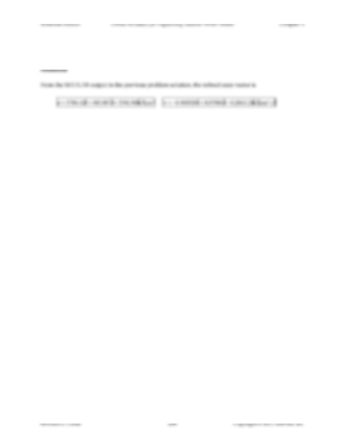
Problem 5.17 Refine the estimate in the previous problem using iterative improvement.
r5788.42ˆ
Problem 5.18 Calculate the orbital elements from the state vector obtained in the previous problem.
Solutions Manual Orbital Mechanics for Engineering Students Third Edition Chapter 5
Howard D. Curtis 210 Copyright © 2013, Elsevier, Inc.
fprintf(‘\n Angular momentum (km^2/s) = %g’, coe(1))
fprintf(‘\n Eccentricity = %g‘, coe(2))
fprintf(‘\n Right ascension (deg) = %g’, coe(3)/deg)
fprintf(‘\n Inclination (deg) = %g’, coe(4)/deg)
fprintf(‘\n Argument of perigee (deg) = %g’, coe(5)/deg)
fprintf(‘\n True anomaly (deg) = %g’, coe(6)/deg)
fprintf(‘\n Semimajor axis (km): = %g’, coe(7))
%...if the orbit is an ellipse, output its period (Equation 2.73):
if coe(2)<1
T = 2*pi/sqrt(mu)*coe(7)^1.5;
fprintf(‘\n Period:‘)
fprintf(‘\n Seconds = %g’, T)
fprintf(‘\n Minutes = %g’, T/60)
fprintf(‘\n Hours = %g’, T/3600)
fprintf(‘\n Days = %g’, T/24/3600)
end
fprintf(‘\n-—–—–——––—–—–—–——–—–——–—–——––—–—–—-\n’)
–—–—–—–——–—––——–—–—––—––——–––——–—–—–
Problem 5.18: Orbital elements from state vector
Gravitational parameter (km^3/s^2) = 398600
State vector:
r (km) = [5788.42 485.007 3341.96]
v (km/s) = [–0.460926 8.0706 –0.266112]
Angular momentum (km^2/s) = 54201.2
Eccentricity = 0.100054
Right ascension (deg) = 270
Inclination (deg) = 30.0001
Argument of perigee (deg) = 89.9993
True anomaly (deg) = 4.15098
Semimajor axis (km): = 7444.75
Period:
Seconds = 6392.73
Minutes = 106.546
Hours = 1.77576
Days = 0.07399
–—–—–—–——–—–——–—–——–––—––—––——–—–——
Orbital elements:
h54 201.2 km 2s
e0.100054
270
i30.0001
89.9993
4.15098