
9-81
When the prior probability of oil is 20%, the optimal policy is to do the survey and drill

9-82
When the prior probability of oil is 30%, the optimal policy is to do the survey and drill

Chapter 09 – Decision Analysis
9-83
When the prior probability of oil is 35%, the optimal policy is to skip the survey and
9-84
Cases
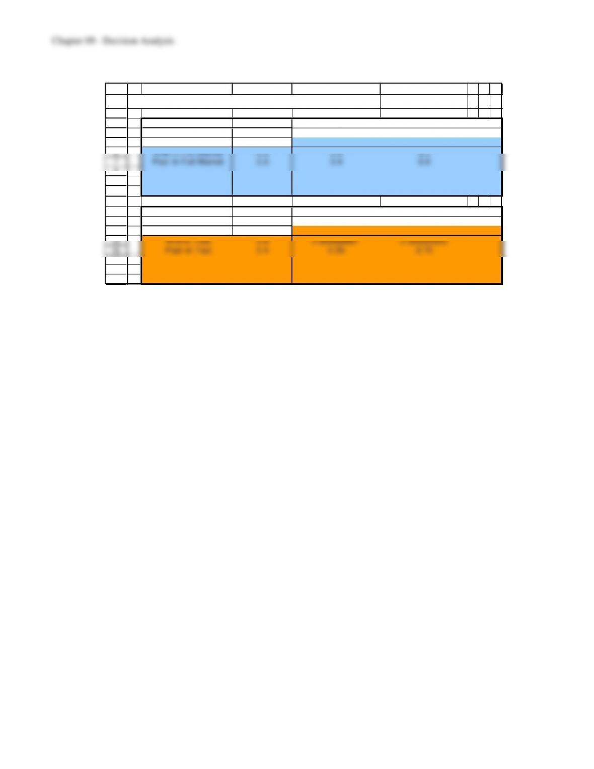
9.1 a) The course of action that maximizes the expected payoff is to answer the $500,000
b) Answers will vary depending on your level of risk aversion. Here is one possible
solution:
a 10% chance of getting $32 thousand, then U($250 thousand) = p = 0.9.

9-85
9-86
9.2 a)
1
2
3
4
5
6
7
8
9
10
11
12
13
14
15
16
17
18
19
A B C D E F G H
Template for Posterior Probabilities
Data:
State of Prior
Nature Probability W ell in Test Poor in Test
W ell in Full Market 0.5 0.8 0.2
Poor in Full Market 0.5 0.4 0.6
Posterior
Prob abilities:
Finding P(Finding) W ell in Full Market Poor in Full Market
W ell in Test 0.6 0.666666667 0.333333333
Poor in Test 0.4 0.25 0.75
P(State | Finding)
State of Nature
P(Finding | State)
Finding

9-87
9-88
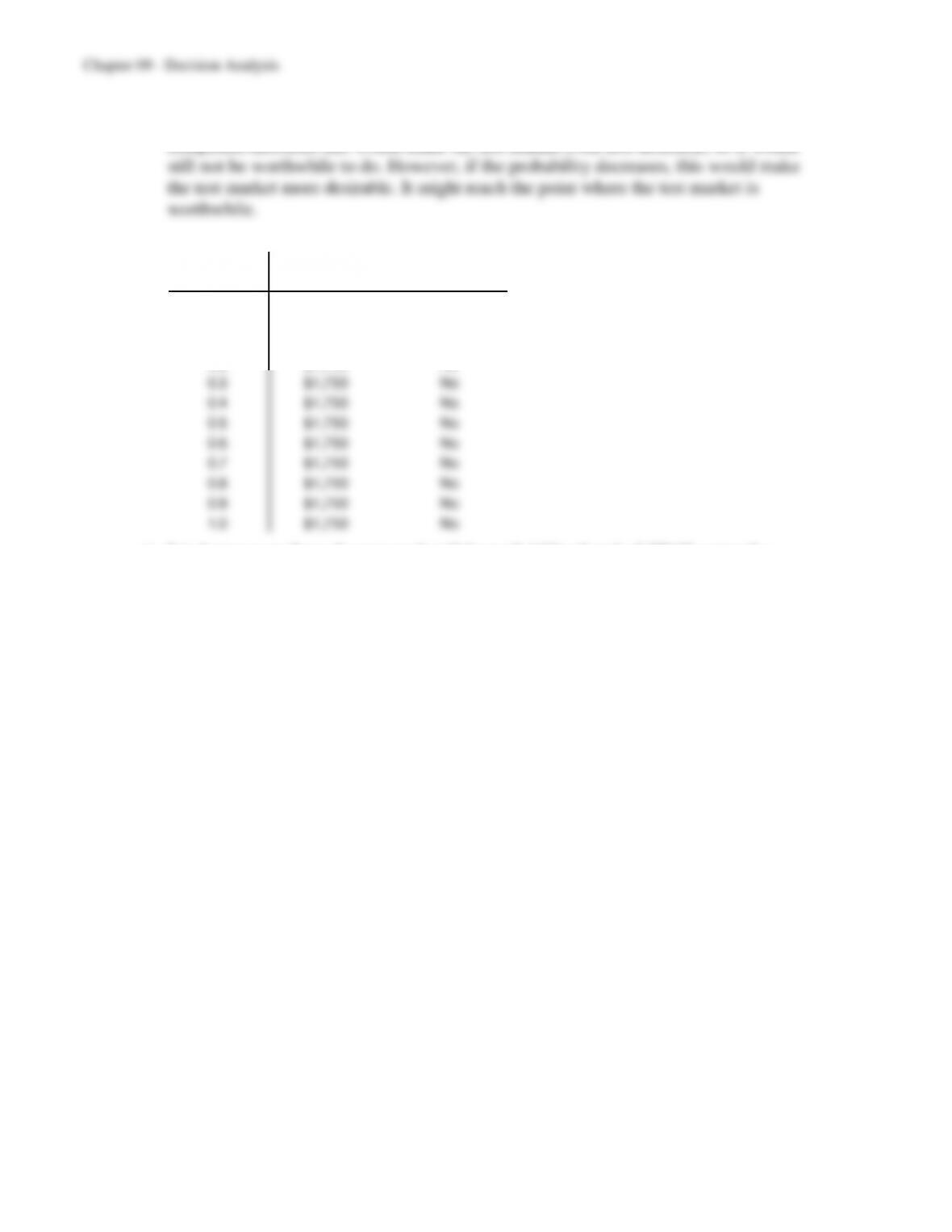
c) If the probability that the LSPAFs enter the market before the test marketing would be
completed increases this would make the test market even less desirable, so it would
d)
Expected Test
Prob(LSPAF) Payoff Market?
$1,750 No
0.0 $1,906 Yes
0.1 $1,755 Yes
0.2 $1,750 No
0.3 $1,750 No
0.4 $1,750 No
0.5 $1,750 No
0.6 $1,750 No
0.7 $1,750 No
0.8 $1,750 No
0.9 $1,750 No
1.0 $1,750 No
e) It is better to perform the test market if the probability that the LSPAFs enter the
market is 10% or less. It is better to skip the test market if the probability is greater than
10%.
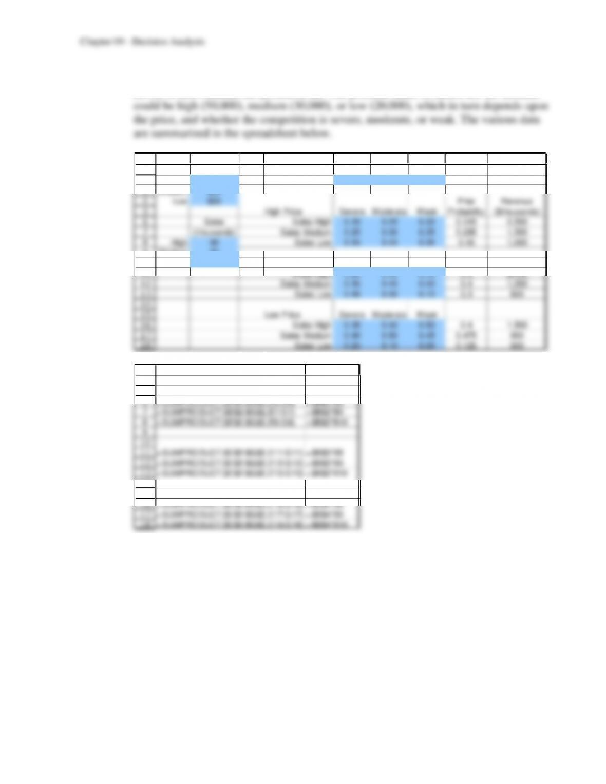
9.3 a) The decision alternatives are to price the product high ($50), medium ($40), or low
($30), or don’t market the product at all. The possible states of nature are the demand
1
2
3
4
5
6
7
8
9
10
11
12
13
14
15
16
17
18
A B C D E F G H I
Price Severe Moderate Weak
High $50 Prior Probability 0.2 0.7 0.1
Medium $40
Low $30 Prior Revenue
High Price Severe Moderate W eak Probability ($thousands)
Sales Sales High 0.20 0.25 0.30 0.245 2,500
(thousands) Sales Medium 0.25 0.30 0.35 0.295 1,500
High 50 Sales Low 0.55 0.45 0.35 0.46 1,000
Medium 30
Low 20 Medium Price Severe Moderate W eak
Sales High 0.25 0.30 0.40 0.3 2,000
Sales Medium 0.35 0.40 0.50 0.4 1,200
Sales Low 0.40 0.30 0.10 0.3 800
Low Price Severe Moderate W eak
Sales High 0.35 0.40 0.50 0.4 1,500
Sales Medium 0.40 0.50 0.45 0.475 900
Sales Low 0.25 0.10 0.05 0.125 600
4
5
6
7
8
9
10
11
12
13
14
15
16
17
18
H I
Prior Revenue
Probability ($thousands)
= SUMPRO DUCT ($E$2: $G $2,E6:G 6) = $B$2*B8
= SUMPRO DUCT ($E$2: $G $2,E7:G 7) = $B$2*B9
= SUMPRO DUCT ($E$2: $G $2,E8:G 8) = $B$2*B10
= SUMPRO DUCT ($E$2: $G $2,E11:G 11) = $B$3*B8
= SUMPRO DUCT ($E$2: $G $2,E12:G 12) = $B$3*B9
= SUMPRO DUCT ($E$2: $G $2,E13:G 13) = $B$3*B10
= SUMPRO DUCT ($E$2: $G $2,E16:G 16) = $B$4*B8
= SUMPRO DUCT ($E$2: $G $2,E17:G 17) = $B$4*B9
= SUMPRO DUCT ($E$2: $G $2,E18:G 18) = $B$4*B10
The payoff table can be generated based on the results in column I.
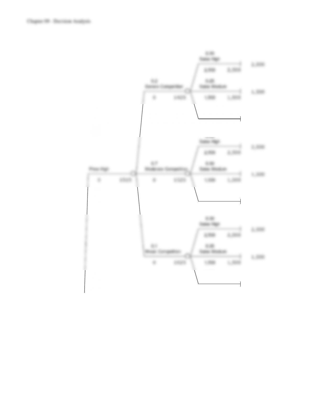
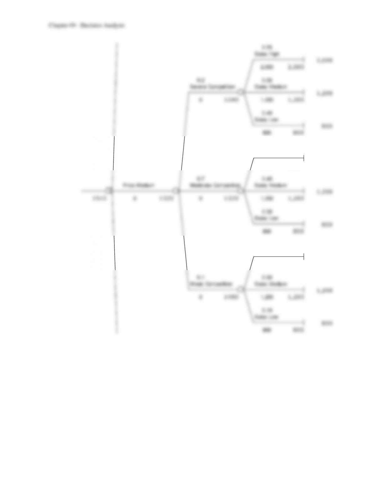
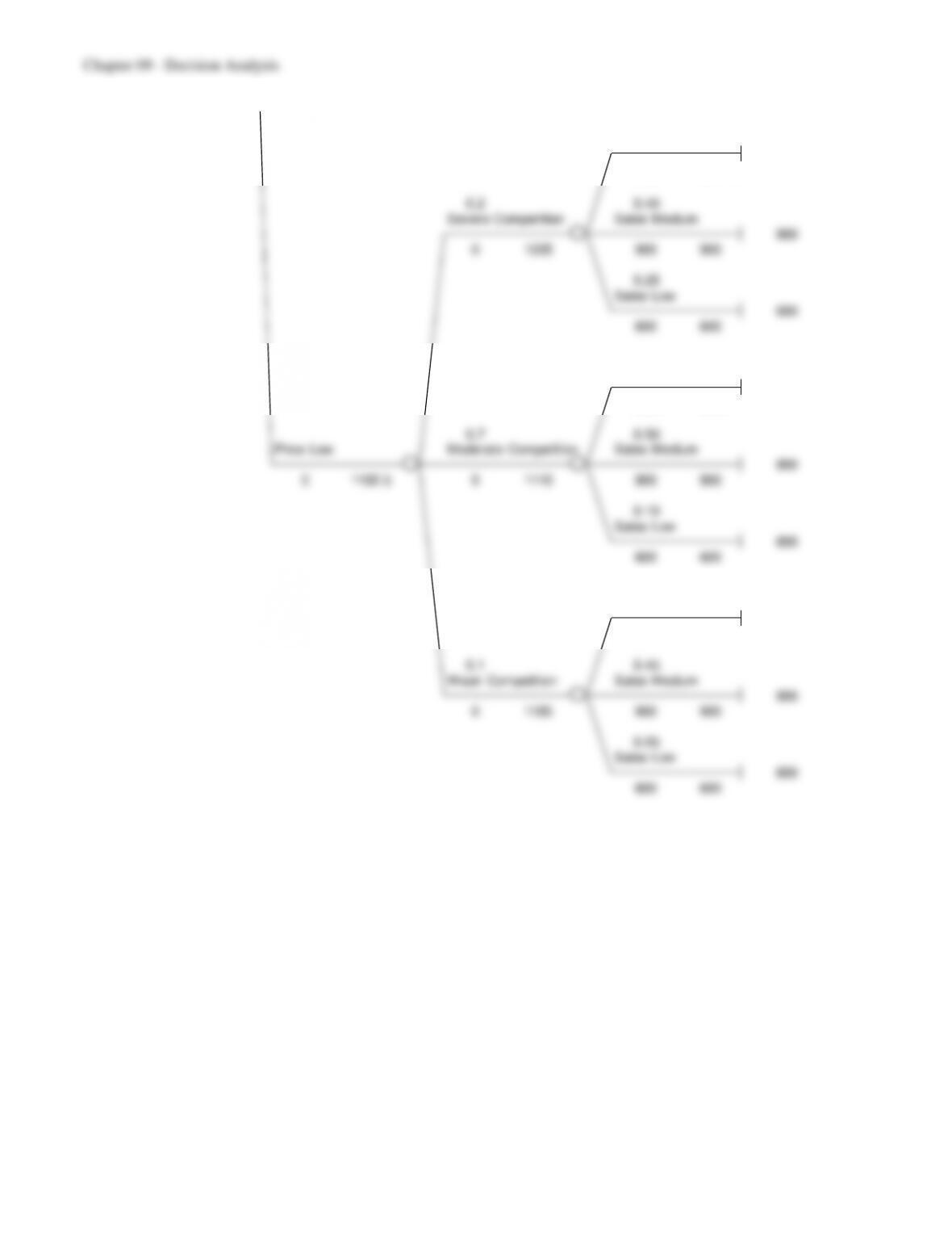
The decision tree for this problem follows (over three pages):
1,000 1,000
0.30
Sales High
2,500
2,500 2,500
1,000 1,000
9-91
0.25
Sales High
2,000
2,000 2,000
0.2 0.35
Severe Competition Sales Medium
1,200
01240 1,200 1,200
0.40
Sales Low
800
800 800
0.30
Sales High
2,000
2,000 2,000
0.7 0.40
Price Medium Moderate Competition Sales Medium
1 1,200
1515 01320 01320 1,200 1,200
0.30
Sales Low
800
800 800
0.40
Sales High
2,000
2,000 2,000
0.1 0.50
W eak Competition Sales Medium
1,200
01480 1,200 1,200
0.10
Sales Low
9-92
0.35
Sales High
1,500
1,500 1,500
0.2 0.40
Severe Competition Sales Medium
900
0 1035 900 900
0.25
Sales Low
600
600 600
0.40
Sales High
1,500
1,500 1,500
0.7 0.50
Price Low Moderate Competition Sales Medium
900
0 1102.5 0 1110 900 900
0.10
Sales Low
600
600 600
0.50
Sales High
1,500
1,500 1,500
0.1 0.45
W eak Competition Sales Medium
900
0 1185 900 900
0.05
Sales Low
600