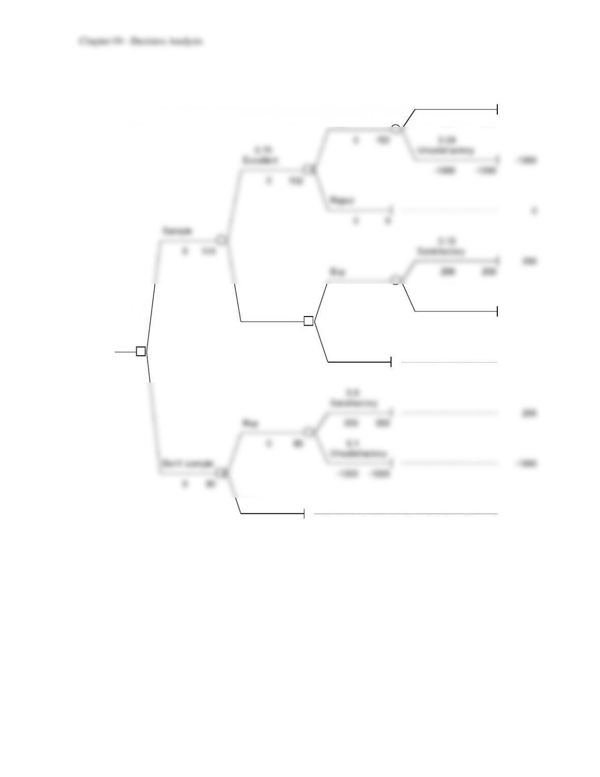
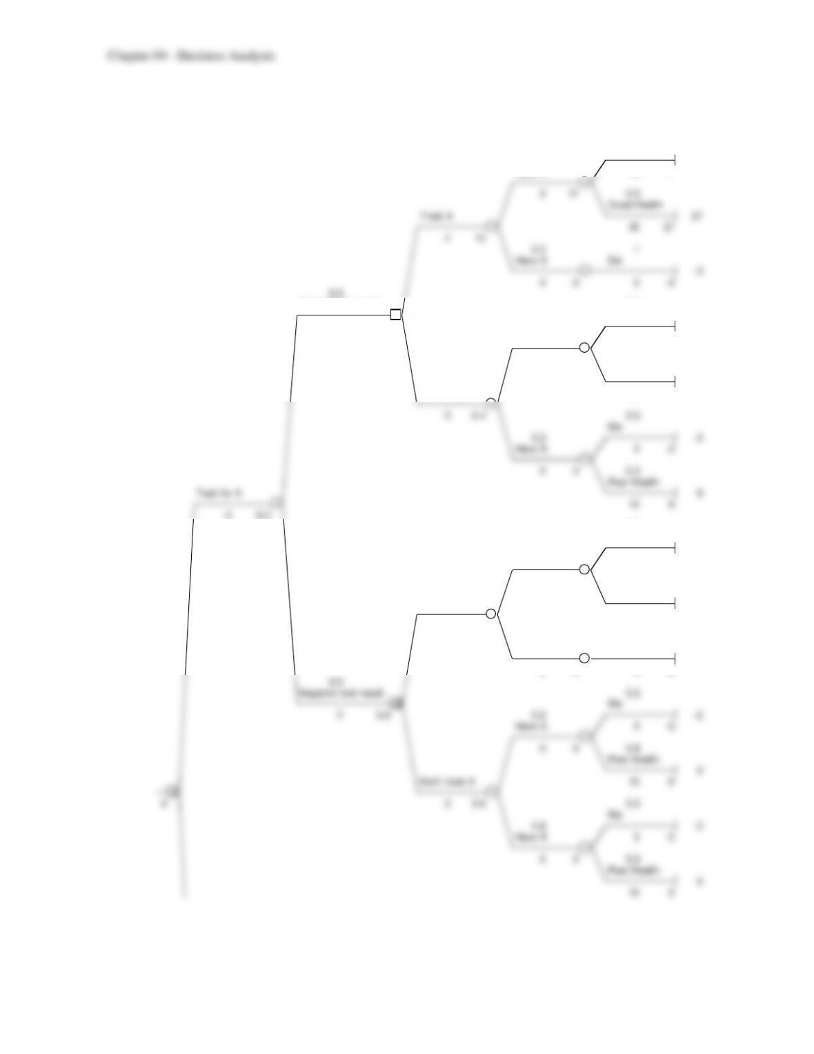
9-61
0.96
Satisfactory
200
Buy 200 200
0 152 0.04
0.75 Unsatisfactory
Excellent –1000
1 -1000 –1000
0 152
Reject
0
0 0
Sample
0.72
0 114 Satisfactory
200
Buy 200 200
0 -136 0.28
0.25 Unsatisfactory
Not Excellent -1000
2 -1000 –1000
0 0
1 Reject
114 0
0 0
0.9
Satisfactory
200
Buy 200 200
080 0.1
Unsatisfactory
Don’t sample -1000
1 -1000 –1000
080
Reject
0
0 0
9-62
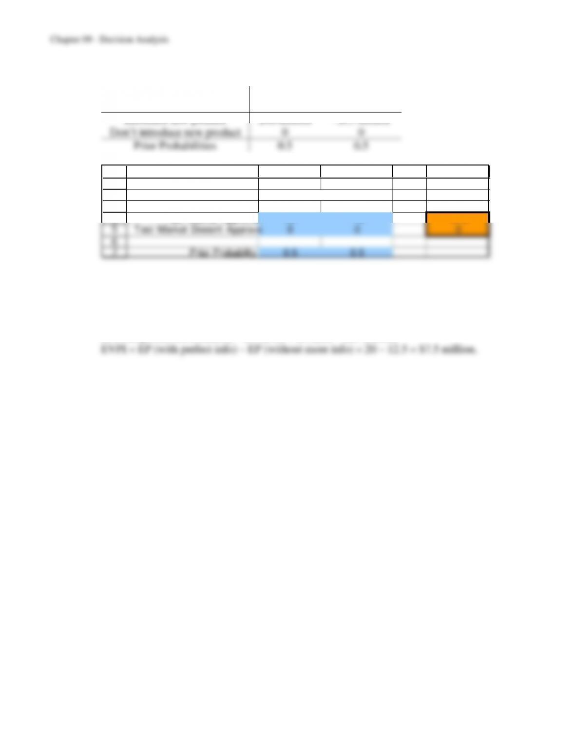
9.31 a)
State of Nature
Alternative
Successful
Unsuccessful
Introduce new product
$40 million
–$15 million
Don’t introduce new product
0
0
Prior Probabilities
0.5
0.5
1
2
3
4
5
6
7
A B C D E
Payoff Table ($millions) Expected
Payoff
Alternative Successful Unsuccessful ($millions)
Test Market Approves 40 -15 12.5
Test Market Doesn’t Approve 0 0 0
Prior Probability 0.5 0.5
State of Nature
Choose to introduce the new product (expected payoff is $12.5 million).
b) With perfect information, Morton Ward should introduce the product if it will be
successful, and don’t introduce the product if it won’t.
EP(with perfect information) = (0.5)(40) + (0.5)(0) = $20 million.
9-63
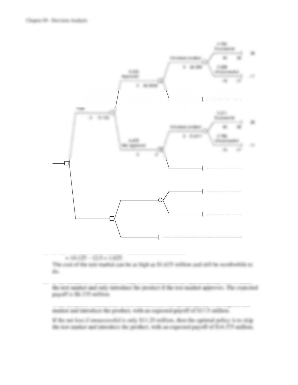
c) The optimal policy is not to test but to introduce the new product. The expected payoff
is $12.5 million.
3
4
5
6
7
8
9
10
11
12
13
14
15
16
17
18
19
B C D E F G H
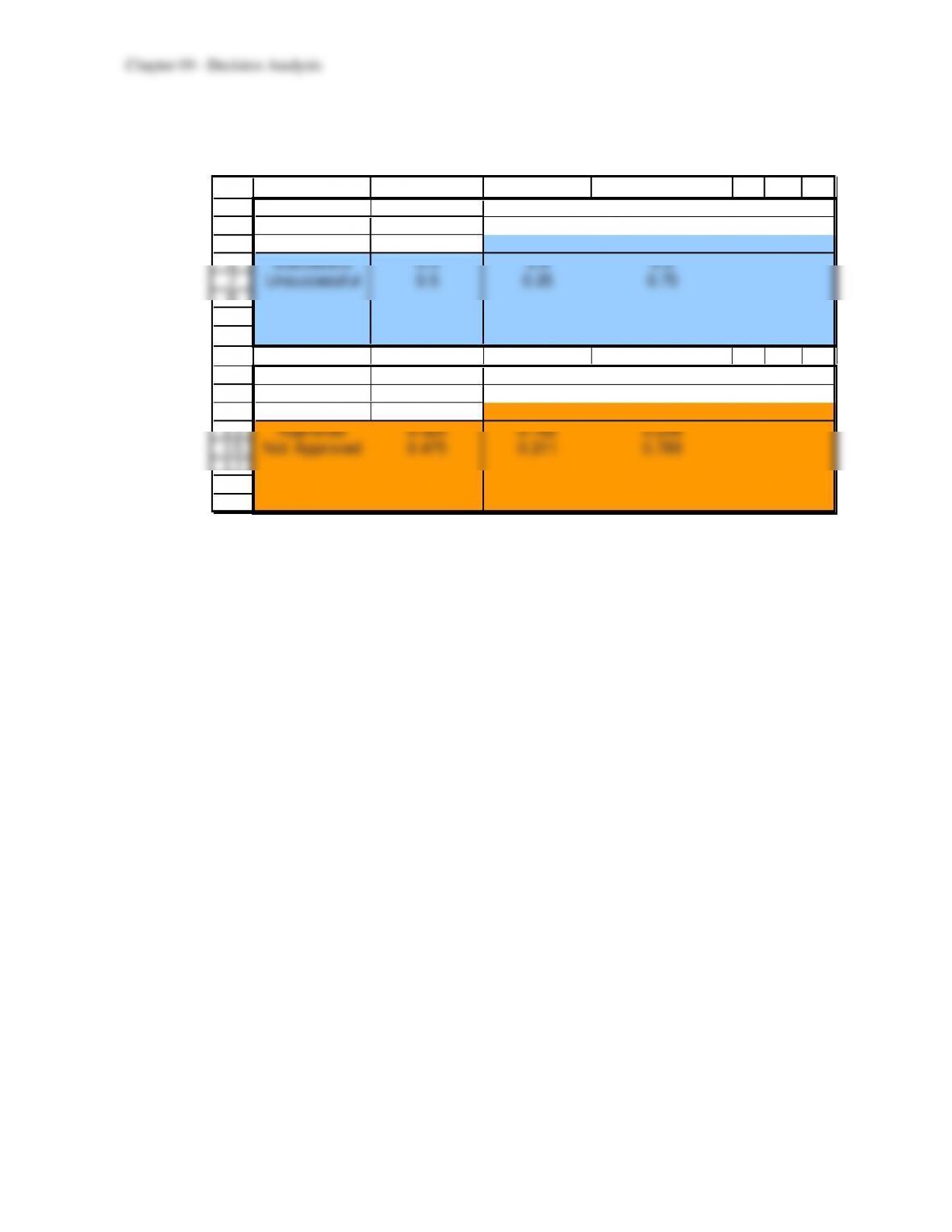
Data:
State of Prior
Nature Probability Approved Not Approved
Successful 0.5 0.8 0.2
Unsuccessful 0.5 0.25 0.75
Posterior
Prob ab i li ties:
Finding P(Finding) Successful Unsuccessful
Approved 0.525 0.762 0.238
Not Approved 0.475 0.211 0.789
P(State | Finding)
State of Nature
P(Finding | State)
Finding
9-65
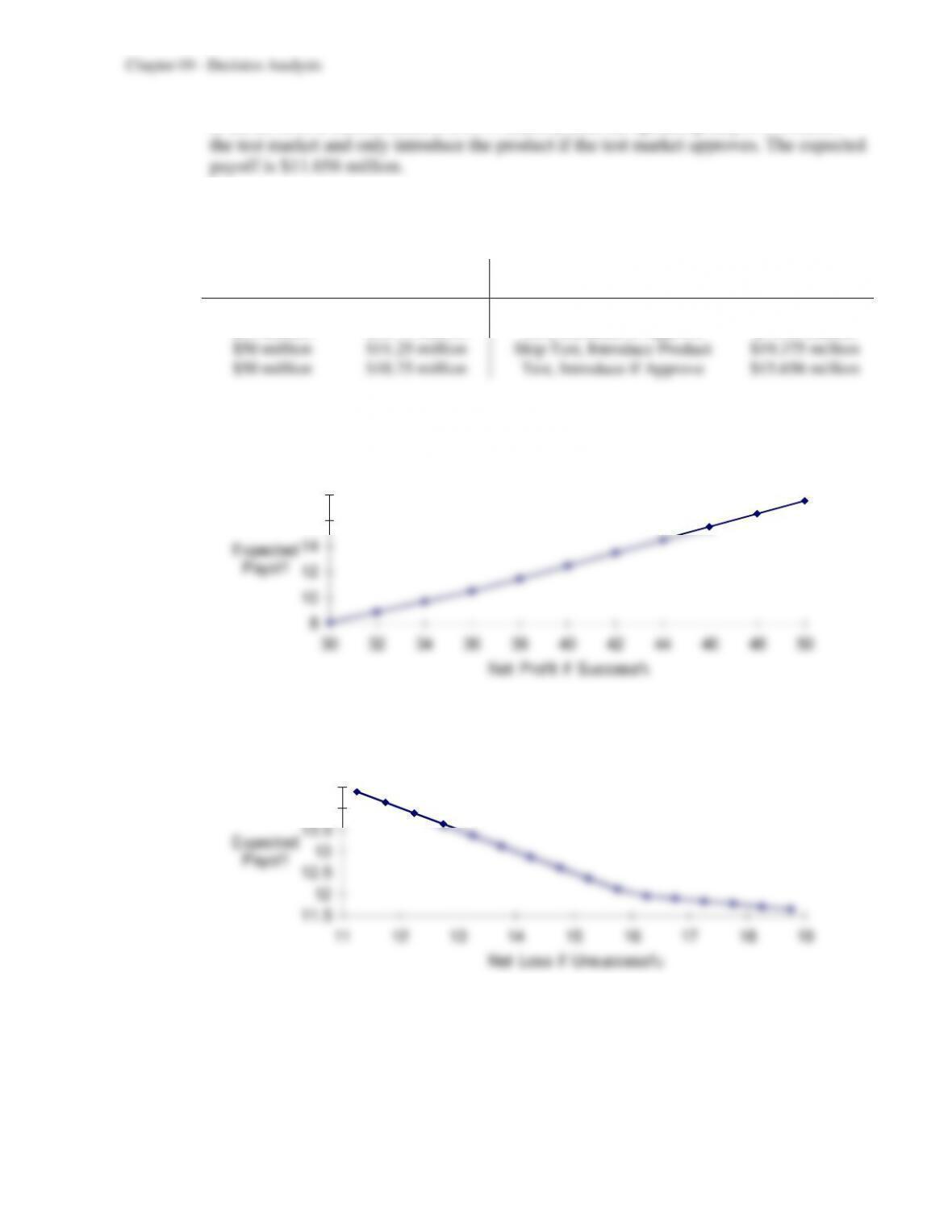
If the net loss if unsuccessful is $18.75 million, then the optimal policy is to conduct
For each combination of financial data, the expected payoff is as shown below. In all
cases, the optimal policy is to build the computers (without market research).
Net Profit if
Successful
Net Loss if
Unsuccessful
Optimal
Policy
Expected
Payoff
$30 million
$11.25 million
Skip Test, Introduce Product
$9.375 million
$30 million
$18.75 million
Test, Introduce if Approve
$7.656 million
$50 million
$11.25 million
Skip Test, Introduce Product
$19.375 million
$50 million
$18.75 million
Test, Introduce if Approve
$15.656 million
f)
Sensit – Sensitivity Analysis – Plo
8
10
12
14
16
18
30 32 34 36 38 40 42 44 46 48 50
Net Profit if Successfu
Expected
Payoff
Sensit – Sensitivity Analysis – Plo
11.5
12
12.5
13
13.5
14
14.5
11 12 13 14 15 16 17 18 19
Net Loss if Unsuccessfu
Expected
Payoff
9-66
g)
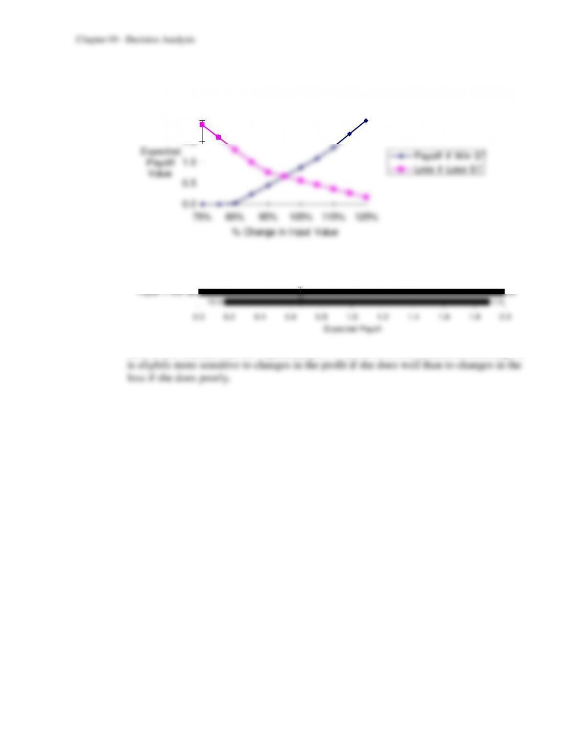
Sensit – Sensitivity Analysis – Spide
8
9
10
11
12
13
14
15
16
17
18
75% 85% 95% 105% 115% 125%
% Change in Input Value
Expected
Payoff
Value
Net Profit if Successful
Net Loss if Unsuccessful
Sensit – Sensitivity Analysis – Tornad
11.25
30
18.75
50
8 9 10 11 12 13 14 15 16 17 18
Net Profit if Successful
Expected Payoff
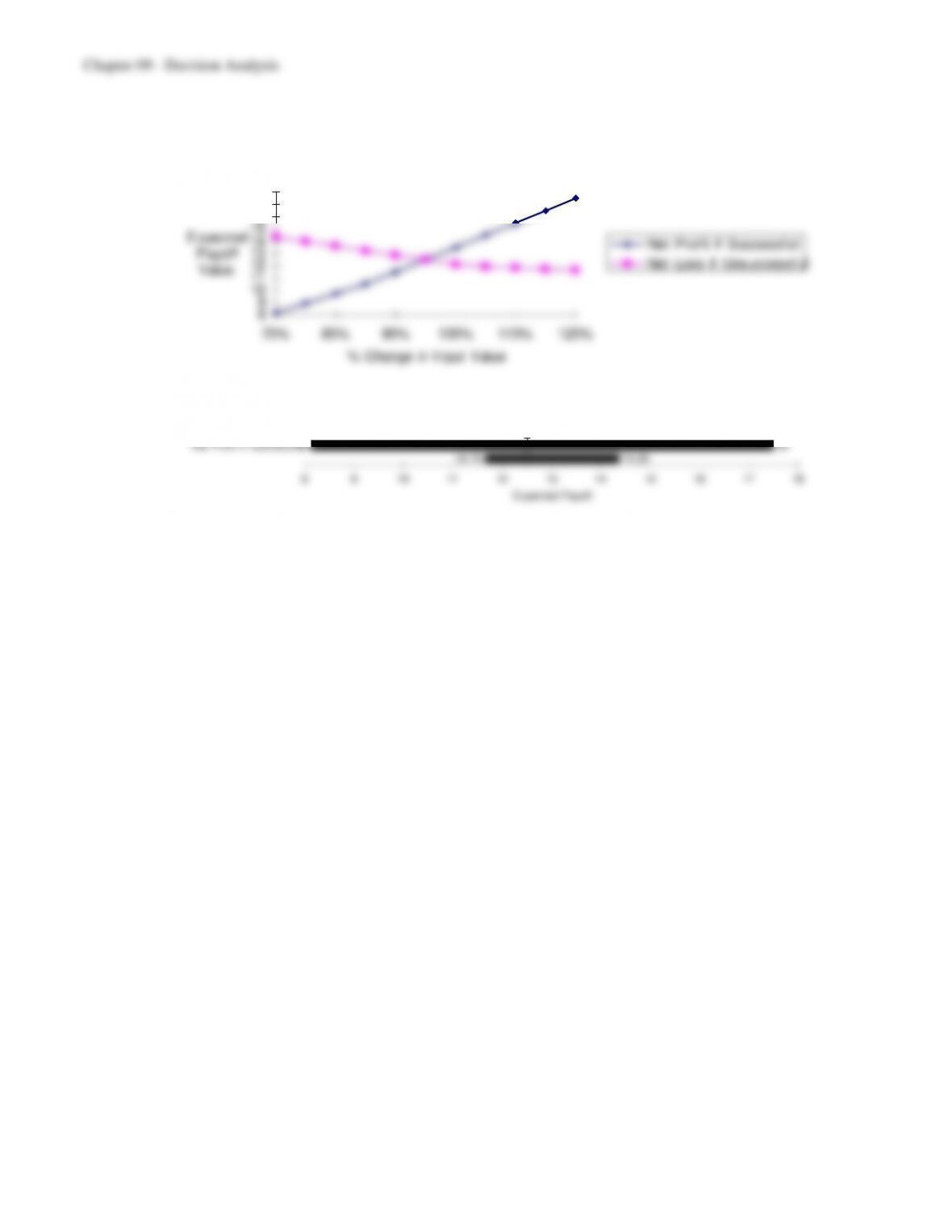
Both charts indicate that the expected profit is sensitive to both parameters, but is
somewhat more sensitive to changes in the profit if successful than to changes in the
loss if unsuccessful.
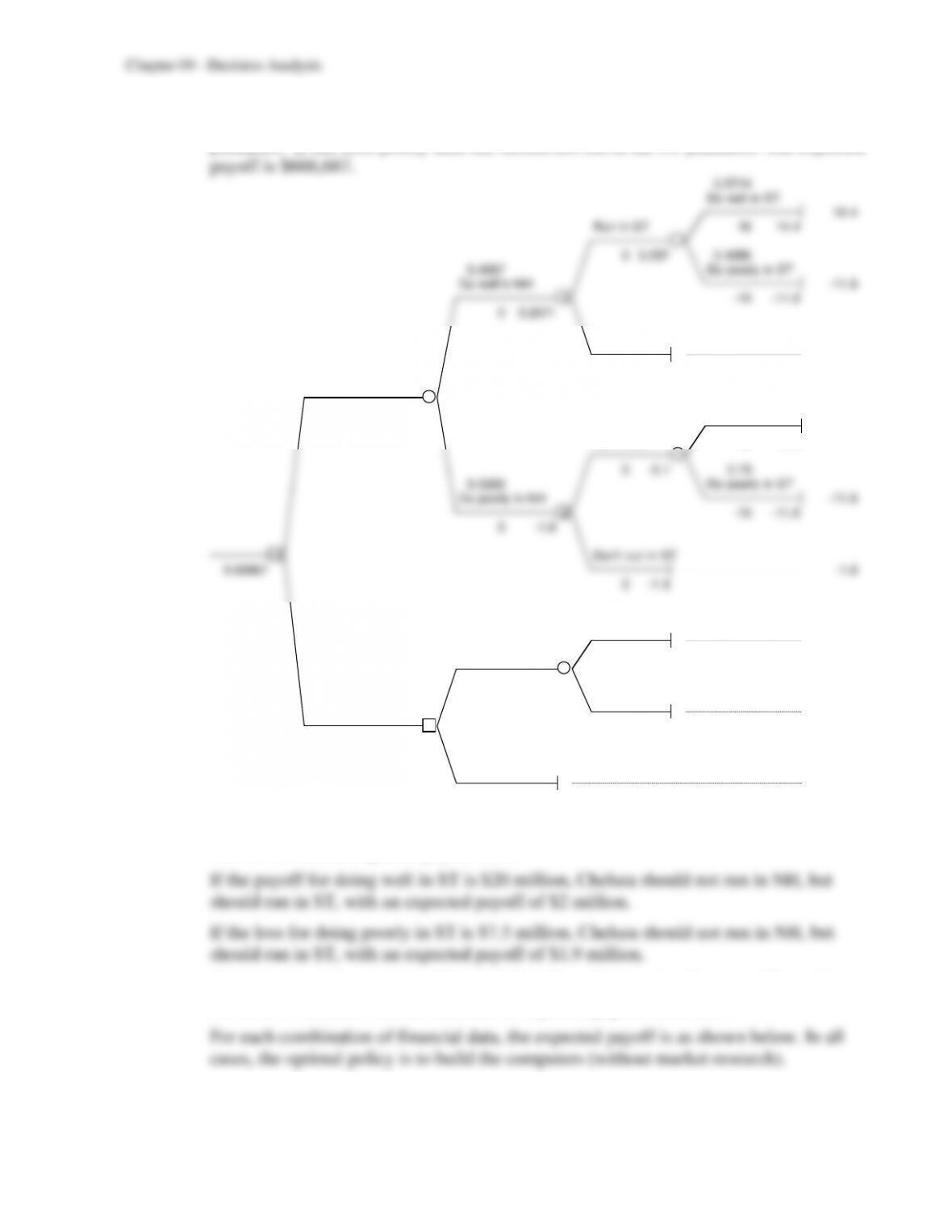
9.32 a) Chelsea should run in the NH primary. If she does well then she should run in the ST
primaries. If she does poorly then she should not run in the ST primaries. The expected
9-68
Payoff if do
Well in ST
Loss if do
Poorly in ST
Optimal
Policy
Expected
Payoff
$12 million
$7.5 million
Run in ST only
$300,000
$12 million
$12.5 million
Don’t run in either
$0
$20 million
$7.5 million
Run in ST only
$3.5 million
$20 million
$12.5 million
Run in NH, Run in ST if do well
$1.233 million
c)
Sensit – Sensitivity Analysis – Plo
0.0
0.5
1.0
1.5
2.0
12 13 14 15 16 17 18 19 20
Payoff if Win ST
Expected
Payoff
Sensit – Sensitivity Analysis – Plo
0
0.5
1
1.5
2
7 8 9 10 11 12 13
Loss if Lose ST
Expected
Payoff
9-69
d)
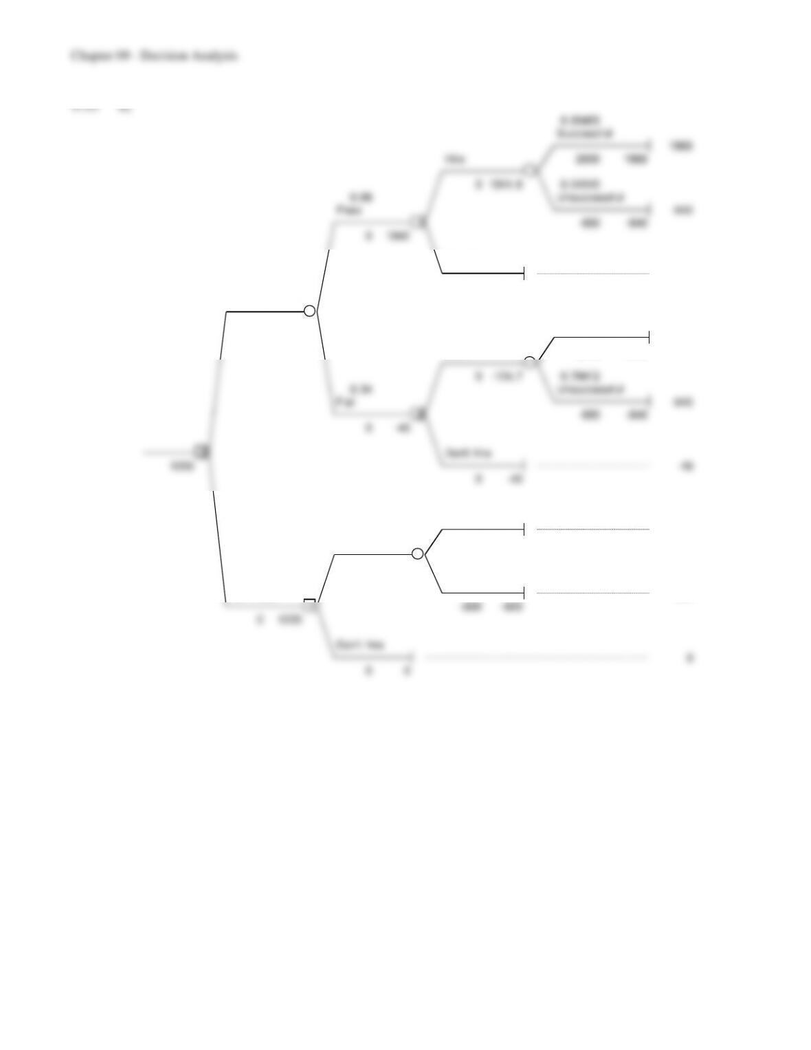
Sensit – Sensitivity Analysis – Spide
0.0
0.5
1.0
1.5
2.0
75% 85% 95% 105% 115% 125%
% Change in Input Value
Expected
Payoff
Value
Payoff if Win ST
Loss if Lose ST
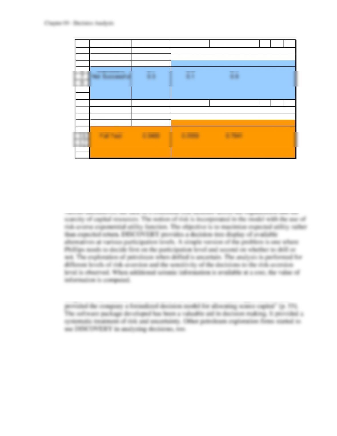
Sensit – Sensitivity Analysis – Tornad
7.5
12
12.5
20
0.0 0.2 0.4 0.6 0.8 1.0 1.2 1.4 1.6 1.8 2.0
Payoff if Win ST
Expected Payoff
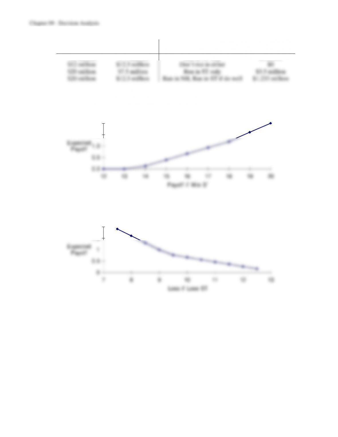
Both charts indicate that the expected payoff is sensitive to both parameters, although it
9-71
3
4
5
6
7
8
9
10
11
12
13
14
15
16
17
18
19
B C D E F G H
Data:
State of Prior
Nature Probability Pass Test Fail Test
Successful 0.7 0.9 0.1
Not Successful 0.3 0.1 0.9
Posterior
Prob ab i li ties:
Finding P(Finding) Successful Not Successful
Pass Test 0.6600 0.9545 0.0455
Fail Test 0.3400 0.2059 0.7941
P(State | Finding)
State of Nature
P(Finding | State)
Finding
The optimal policy is not to pay for testing and to hire Matthew.
b) If the fee is less than $22,000 then the testing is worthwhile.
9.34 Phillips Petroleum Company developed a decision analysis tool named DISCOVERY to
evaluate available investment opportunities and decide on the participation levels. The
need for a systematic decision analysis tool arose from the uncertainty associated with
This study “has increased management’s awareness of risk and risk tolerance, provided
insight into the financial risks associated with its set of investment opportunities, and
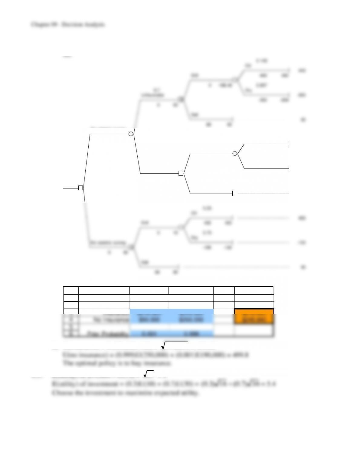
9.35 a & b) They should do no seismic survey, and sell the land, with an expected utility of
9-73
9.38 U(10) = 0, U(30) = 1.
U(19) = p such that you are indifferent between 30 with probability p and 10 with
9.39 a) U(1) = p = 0.125.
9.40 a) Expected utility of A1 = pU(25) + (1 – p)U(36) = 5p + 6(1 – p) = 6 – p.
9-74
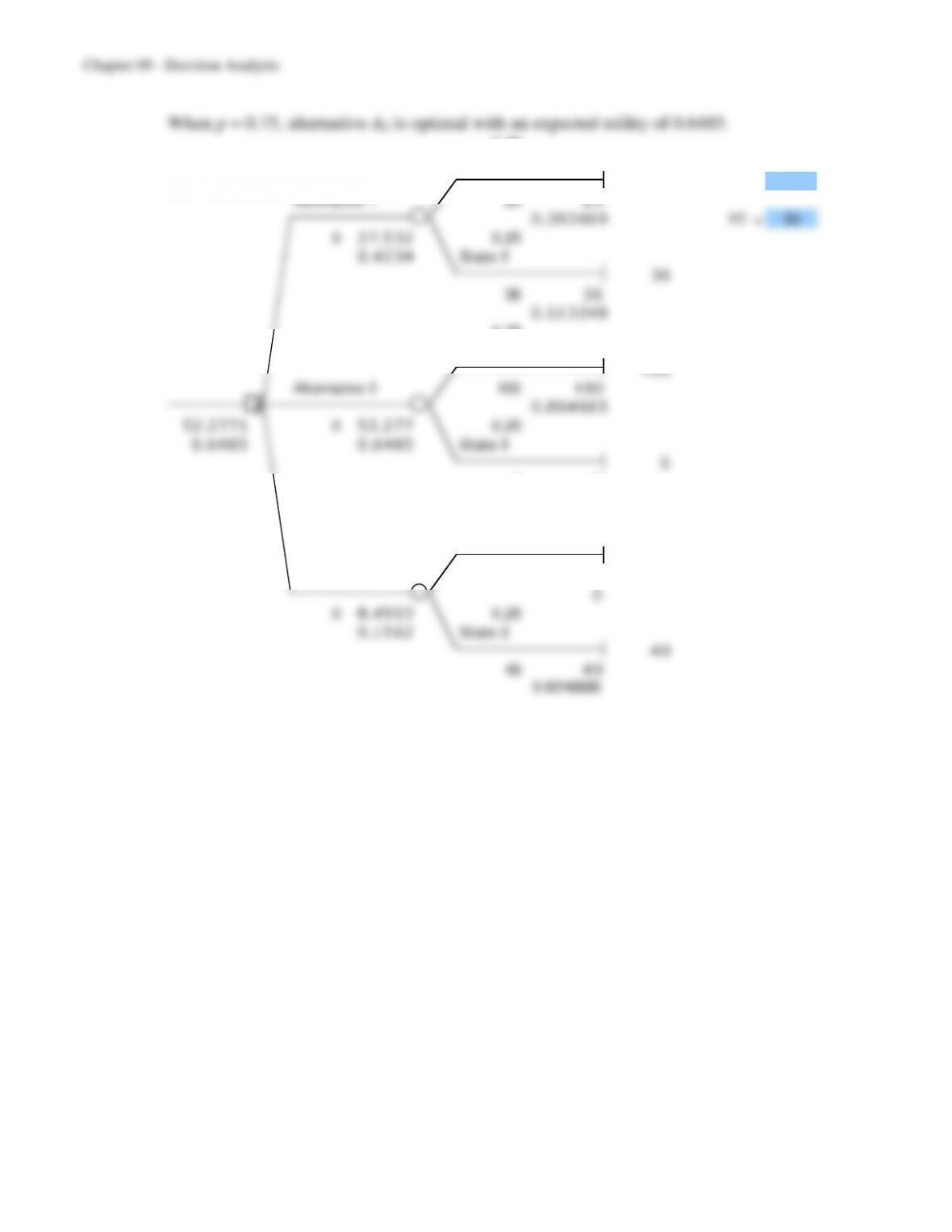
b) When p = 0.25, alternative A1 is optimal with an expected utility of 0.4833.
0.25
State 1
25 p= 0.25
Alternative 1 25 25
0.39 3 46 9 RT = 50
033.0 1 5 0.75
0.48 3 3 State 2
36
36 36
0.51 3 24 8
0.25
State 1
100
Alternative 2 100 100
1 0.86 4 66 5
33.0 1 49 01 2.178 0.75
0.48 3 3 0.21 6 2 State 2
0
00
0
0.25
State 1
0
Alternative 3 0 0
0
031.6 0 4 0.75
0.46 8 5 State 2
49
49 49
0.6246889
9-75
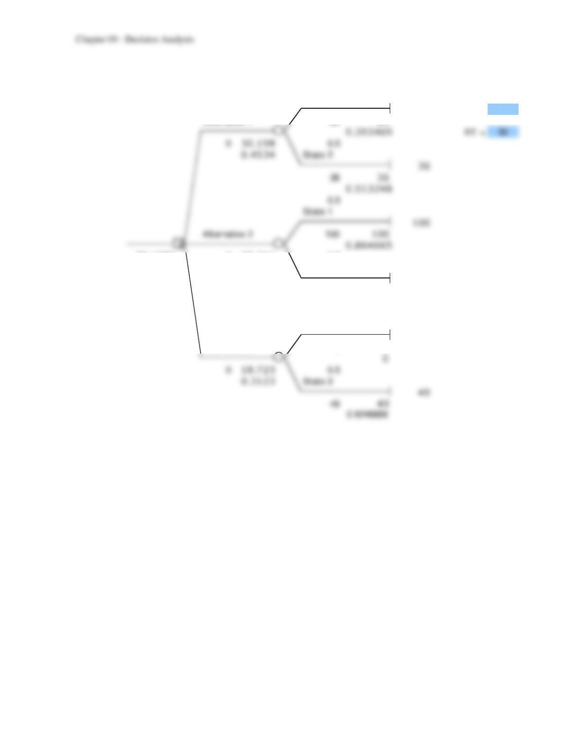
When p = 0.5, alternative A1 is optimal with an expected utility of 0.4534.
0.5
State 1
25 p= 0.5
Alternative 1 25 25
0.39 3 46 9 RT = 50
030.1 9 8 0.5
0.45 3 4 State 2
36
36 36
0.51 3 24 8
0.5
State 1
100
Alternative 2 100 100
1 0.86 4 66 5
30.1 9 81 02 8.311 0.5
0.45 3 36 0.43 2 3 State 2
0
00
0
0.5
State 1
0
Alternative 3 0 0
0
018.7 2 3 0.5
0.31 2 3 State 2
49
49 49
0.6246889
9-76
0.75
State 1
25 p= 0.75
Alternative 1 25 25
0.39 3 46 9 RT = 50
027.5 3 2 0.25
0.42 3 4 State 2
36
36 36
0.51 3 24 8
0.75
State 1
100
Alternative 2 100 100
2 0.86 4 66 5
52.2 7 71 05 2.277 0.25
0.64 8 5 0.64 8 5 State 2
0
00
0
0.75
State 1
0
Alternative 3 0 0
0
08.49 0 3 0.25
0.15 6 2 State 2
49
49 49
0.6246889
9-77
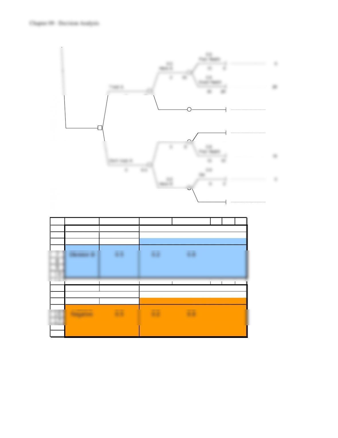
9.41 The optimal policy is not to test for disease A but to treat disease A. (Note: this decision
tree is continued on the next page.)
0.5
Poor Health
0.8 7
Have A 10 7
017 0.5
Good Health
Treat A 27
30 27
-1 13
0.2 1
Have B Die
-3
0-3 0-3
0.5
Positive test result 0.2
1 Die
013 0.8 -2
Have A 0 -2
0 6 0.8
Poor Health
8
Don’t treat A 10 8
0 5.4 0.5
Die
0.2 -2
Have B 0 -2
0 3 0.5
Poor Health
Test for A 8
10 8
-2 8.3
0.5
Poor Health
0.2 7
Have A 10 7
017 0.5
Good Health
Treat A 27
30 27
-1 1
0.8 1
Have B Die
-3
0-3 0-3
0.5
Negative test result 0.2
2 Die
0 3.6 0.2 -2
Have A 0 -2
0 6 0.8
Poor Health
8
Don’t treat A 10 8
2
9 0 3.6 0.5
Die
0.8 -2
Have B 0 -2
0 3 0.5
Poor Health
8
10 8
9-78
0.5
Poor Health
0.5 9
Have A 10 9
019 0.5
Good Health
Treat A 29
30 29
-1 9
0.5 1
Have B Die
-1
0-1 0-1
Don’t test for A 0.2
1 Die
0 9 0.5 0
Have A 0 0
0 8 0.8
Poor Health
10
Don’t treat A 10 10
0 6.5 0.5
Die
0.5 0
Have B 0 0
0 5 0.5
Poor Health
10
10 10
3
4
5
6
7
8
9
10
11
12
13
14
15
16
17
18
19
B C D E F G H
Data:
State of Prior
Nature Probability Positive Negative
Disease A 0.5 0.8 0.2
Disease B 0.5 0.2 0.8
Po sterio r
Prob ab il iti es:
Finding P(Finding) Disease A Disease B
Positive 0.5 0.8 0.2
Negative 0.5 0.2 0.8
P(State | Finding)
State of Nature
P(Finding | State)
Finding
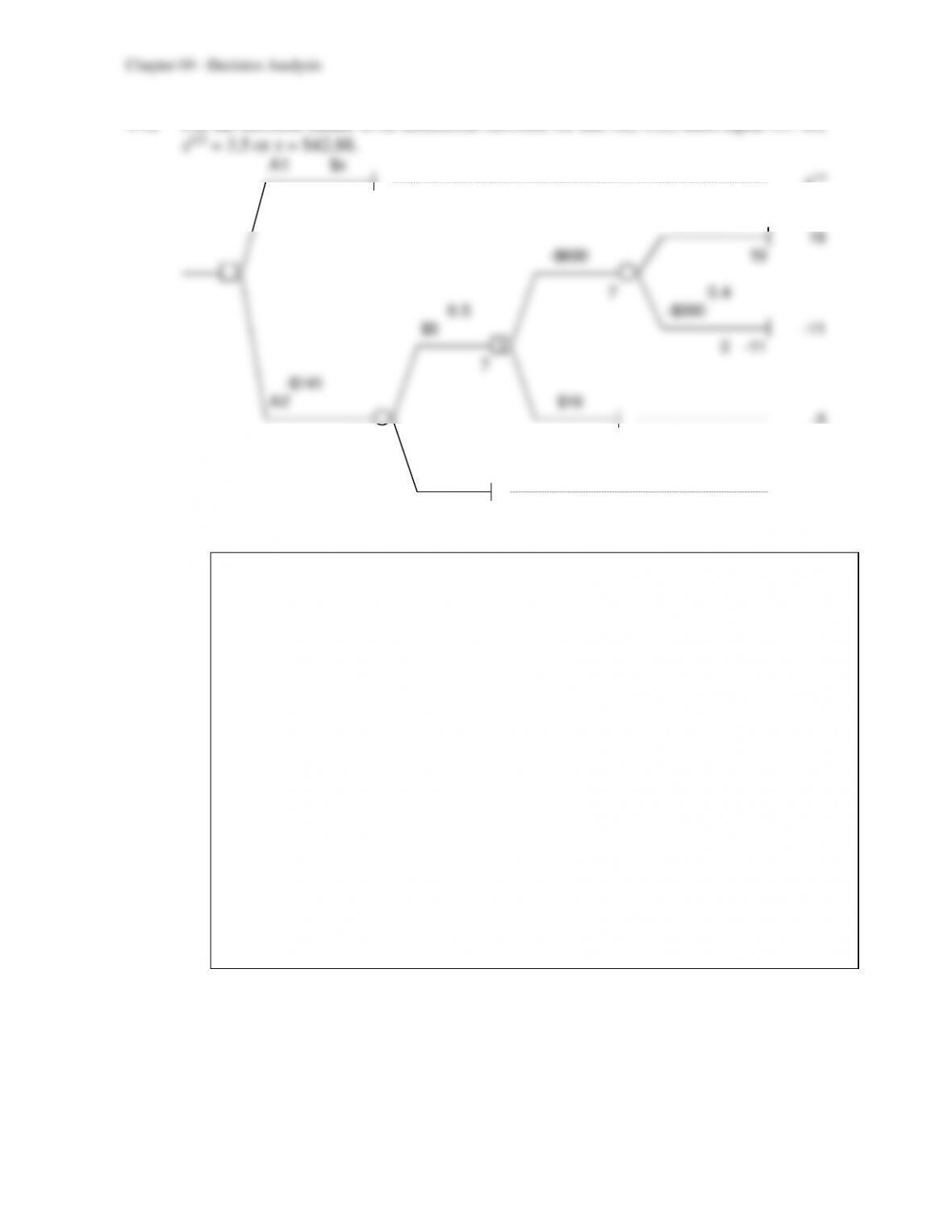
9.42 For the decision-maker to be indifferent between A1 and A2, U(x) must equal 3.5. So,

9-80
b) When the prior probability of oil is 15%, the optimal policy is to do no survey and sell