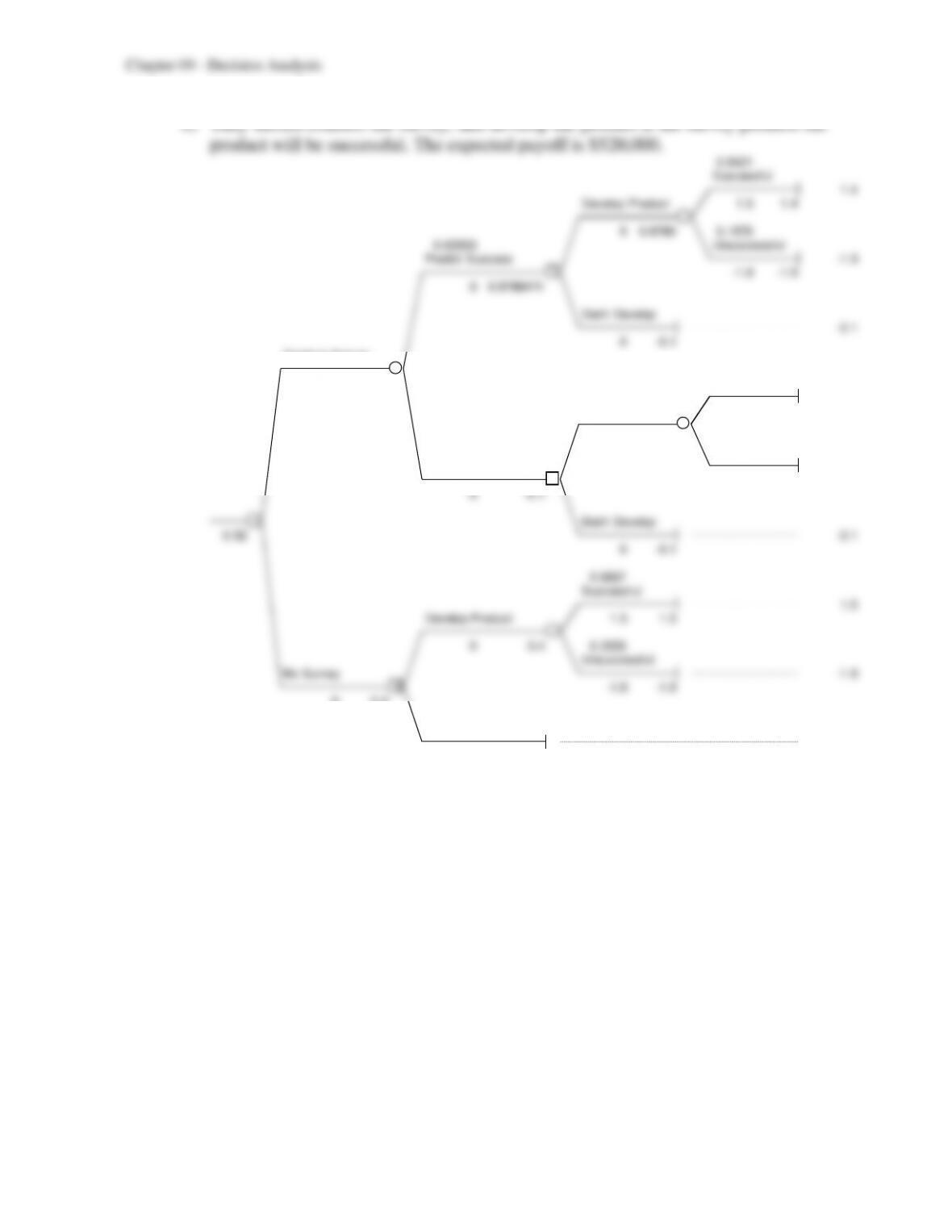
e) They should conduct the survey, and develop the product if the survey predicts the
9-42
f)
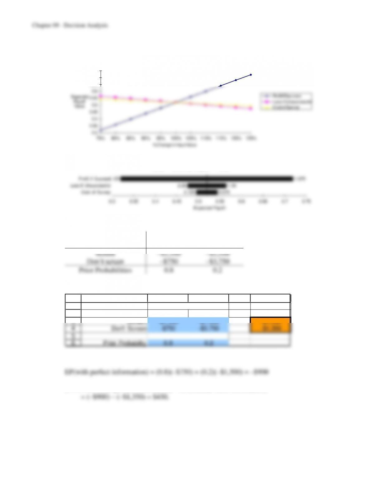
Sensit – Sensitivity Analysis – Spider
0.3
0.35
0.4
0.45
0.5
0.55
0.6
0.65
0.7
0.75
75% 80% 85% 90% 95% 100% 105% 110% 115% 120% 125%
% Change in Input Value
Expected
Payoff
Value
Profit if Success
Loss if Unsuccessful
Cost of Survey
Sensit – Sensitivity Analysis – Tornad
0.075
1.35
1.125
0.125
2.25
1.875
0.3 0.35 0.4 0.45 0.5 0.55 0.6 0.65 0.7 0.75
Profit if Success
Loss if Unsuccessful
Cost of Survey
Expected Payoff
9.21 a)
State of Nature
Alternative
p=0.05
p=0.25
Screen
–$1,500
–$1,500
Don’t screen
–$750
–$3,750
Prior Probabilities
0.8
0.2
b) Choosing not to screen maximizes the expected payoff. The expected cost is $1,350.
1
2
3
4
5
6
A B C D E
Payoff Table Expected
Alternative p = 0.05 p = 0.25 Payoff
Screen -$1,500 –$1,500 -$1,500
Don‘t Screen -$750 -$3,750 -$1,350
Prior Probability 0.8 0.2
State of Nature
c) With perfect information, they would screen if p = 0.25, and don’t screen if p = 0.05.
EVPI = EP(with perfect information) – EP(without more information)
This indicates that consideration should be given to inspecting the single item.
9-43
d)
3
4
5
6
7
8
9
10
11
12
13
14
15
16
17
18
19
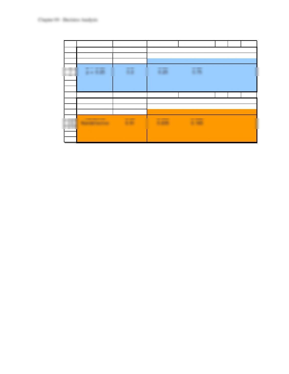
B C D E F G H
Data:
State of Prior
Nature Probability Defective Nondefective
p = 0.05 0.8 0.05 0.95
p = 0.25 0.2 0.25 0.75
Po sterior
Prob ab il iti es:
Finding P(Finding) p = 0.05 p = 0.25
Defective 0.09 0.444 0.556
Nondefective 0.91 0.835 0.165
P(State | Finding)
State of Nature
P(Finding | State)
Finding
9-44
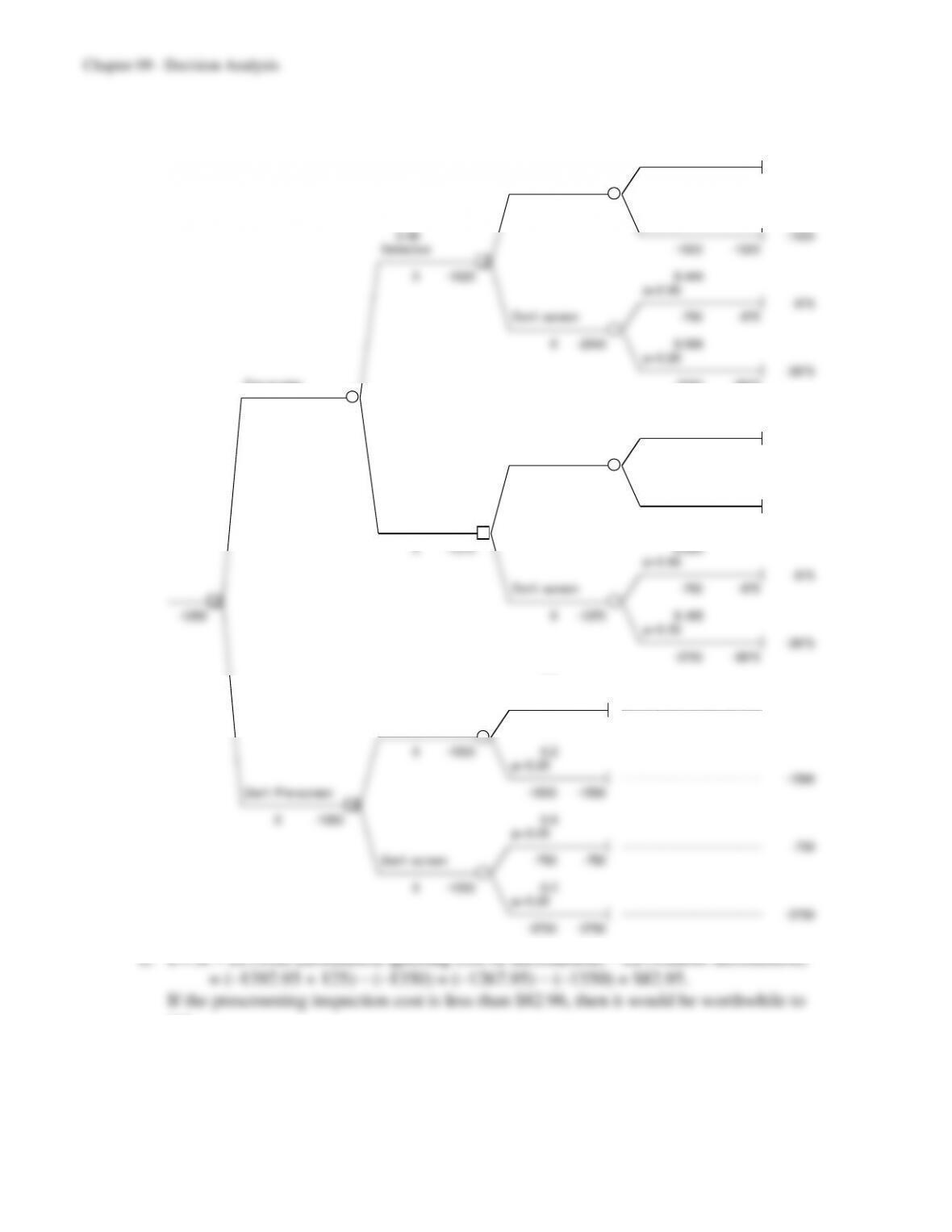
e) The optimal policy is not to pre-screen or screen.
0.444
p= 0.05
-1625
Screen -1500 -1625
0 -1625 0.556
p= 0.25
0.09 -1625
Defective -1500 -1625
1
0 -1625 0.444
p= 0.05
-875
Don’t screen -750 -875
0 -2543 0.556
p= 0.25
-3875
Pre-screen -3750 -3875
-125 -1392.95 0.835
p= 0.05
-1625
Screen -1500 -1625
0 -1625 0.165
p= 0.25
0.91 -1625
Nondefective -1500 -1625
2
0 -1370 0.835
p= 0.05
-875
Don’t screen -750 -875
2
-1350 0 -1370 0.165
p= 0.25
-3875
-3750 -3875
0.8
p= 0.05
-1500
Screen -1500 -1500
0 -1500 0.2
p= 0.25
-1500
Don’t Pre-screen -1500 -1500
2
0 -1350 0.8
p= 0.05
-750
Don’t screen -750 –750
0 -1350 0.2
p= 0.25
-3750
-3750 -3750
f) EVSI = EP(with information ignoring cost of information) – EP(without information)
use.
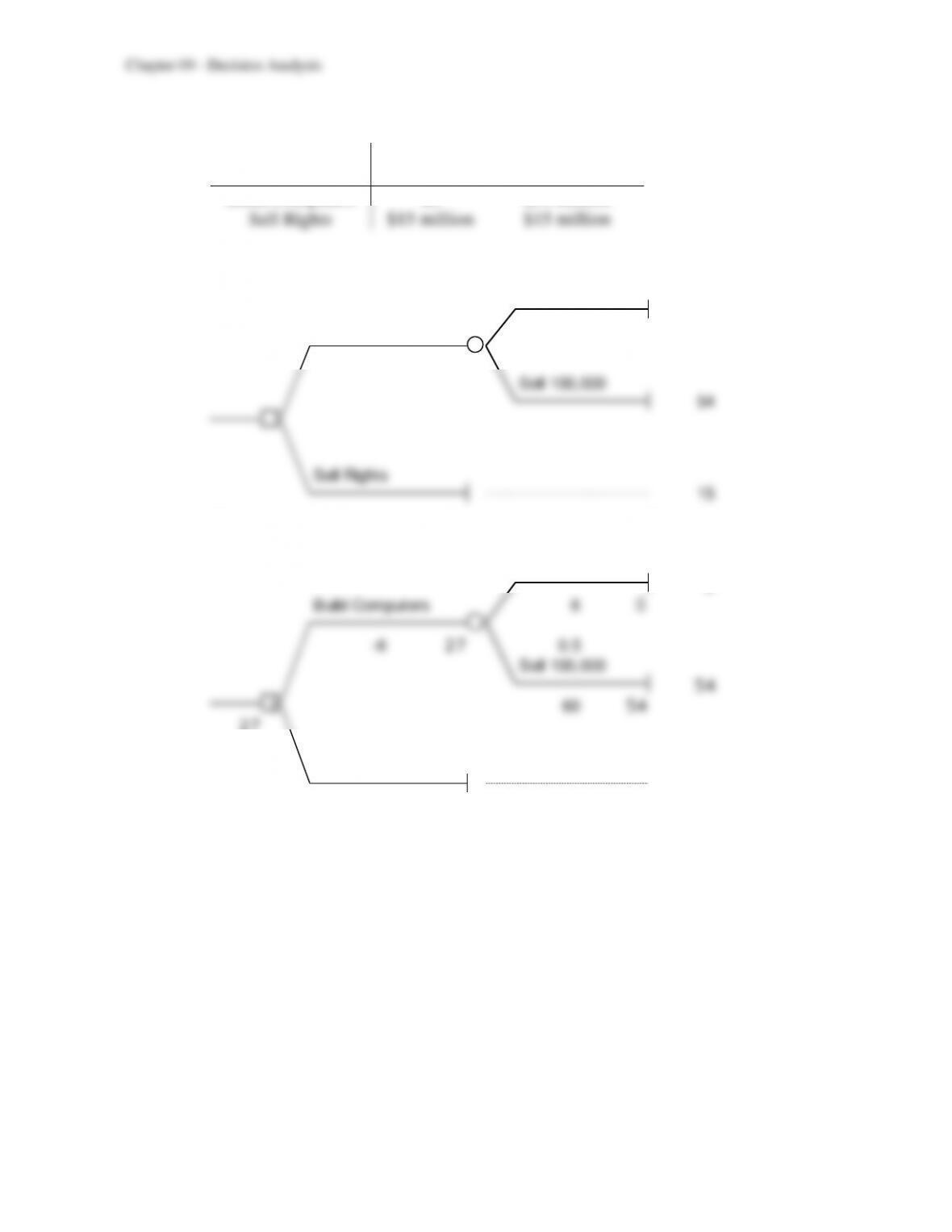
9.22 a)
State of Nature
Alternative
Sell 10,000
Sell 100,000
Build Computers
$0
$54 million
Sell Rights
$15 million
$15 million
b)
Sell 10,000
0
Build Computers
Sell 100,000
54
Sell Rights
15
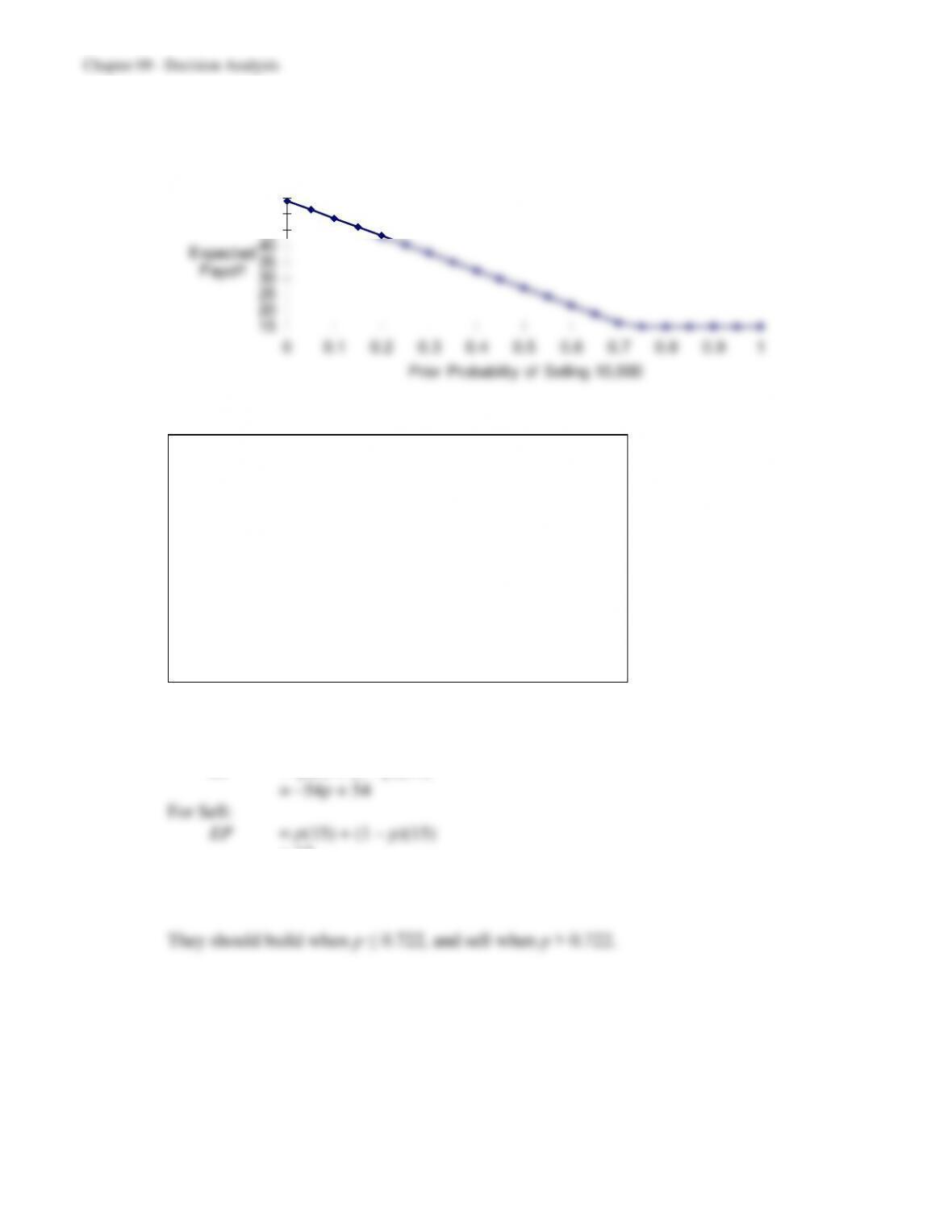
c) They should build computers, with an expected payoff of $27 million.
0.5
Sell 10,000
0
Build Computers 6 0
-6 27 0.5
Sell 100,000
54
160 54
27
Sell Rights
15
15 15
9-46
d)
Sensit – Sensitivity Analysis – Plo
15
20
25
30
35
40
45
50
55
0 0.1 0.2 0.3 0.4 0.5 0.6 0.7 0.8 0.9 1
Prior Probability of Selling 10,000
Expected
Payoff
e)
f) Let p = prior probability of selling 10,000.
For Build:
EP = p(0) + (1 – p)(54)
= 15
Build and Sell cross when –54p + 54 = 15 or 54p = 39 or p = 0.722

9-47
9.23 a) With perfect information, they should build computers if they will sell 100,000 of them,
and sell the rights if they could only sell 10,000 computers.
EVPI = EP(with perfect information) – EP without more information)
b) Since the market research will cost $1 million it might be worthwhile to perform it.
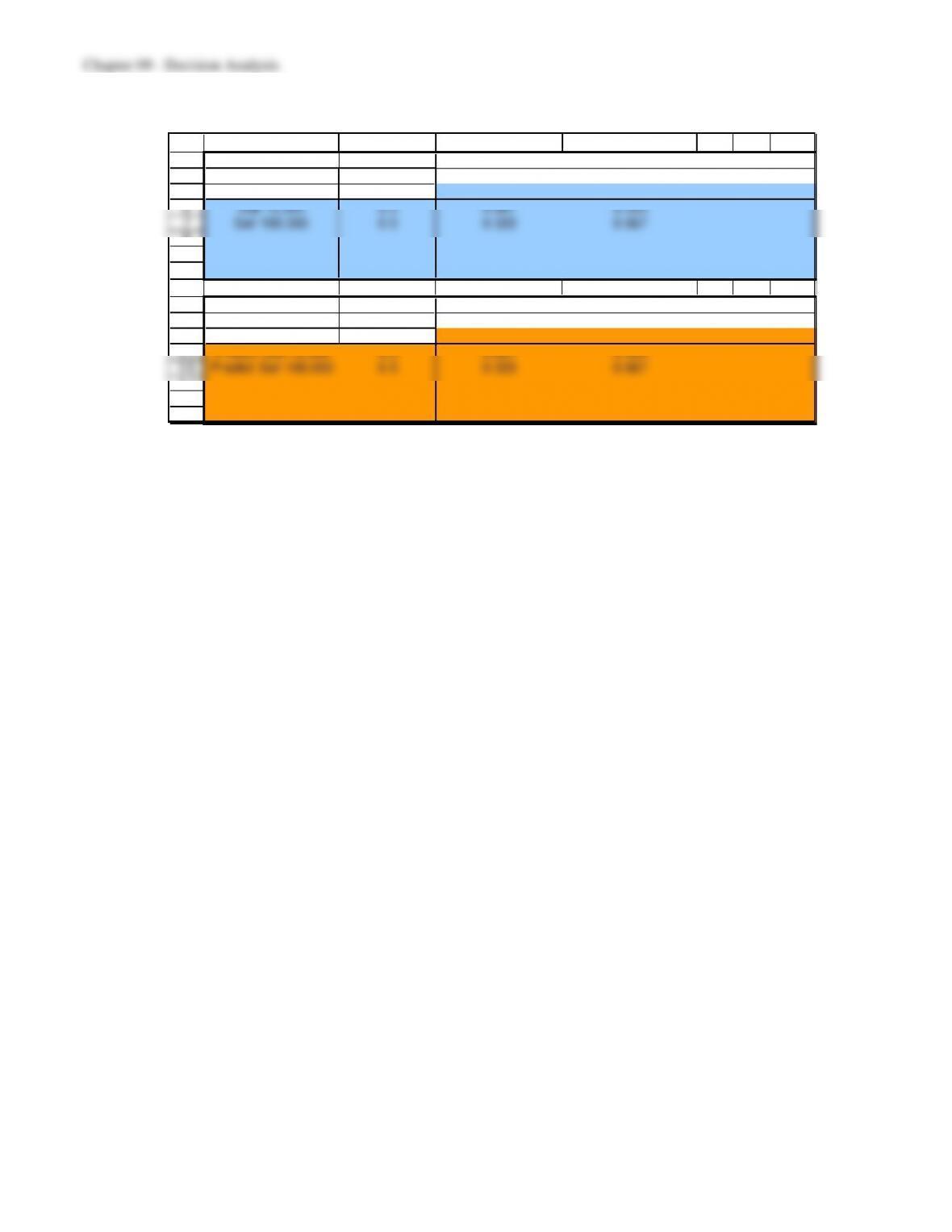
c)
9-48
d)
3
4
5
6
7
8
9
10
11
12
13
14
15
16
17
18
19
B C D E F G H
Data:
State of Prior
Nature Probability Predict Sell 10,000 Predict Sell 100,000
Sell 10,000 0.5 0.667 0.333
Sell 100,000 0.5 0.333 0.667
Posterior
Prob ab il i ties:
Finding P(Finding) Sell 10,000 Sell 100,000
Predict Sell 10,000 0.5 0.667 0.333
Predict Sell 100,000 0.5 0.333 0.667
P(State | Finding)
State of Nature
P(Finding | State)
Finding
9-49
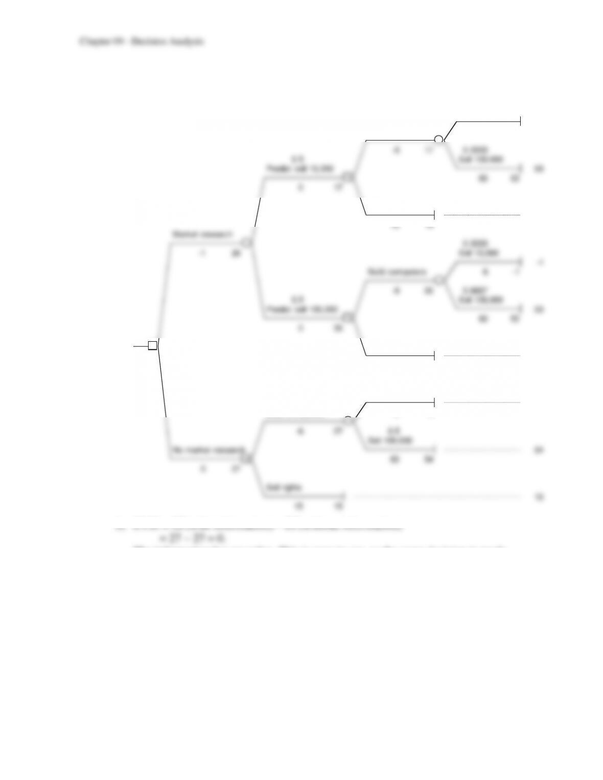
9.24 a) The optimal policy is to do no market research and build the computers. The expected
payoff is $27 million.
0.6667
Sell 10,000
-1
Build computers 6 -1
-6 17 0.3333
0.5 Sell 100,000
Predict sell 10,000 53
160 53
017
Sell rights
14
15 14
Market research
0.3333
-1 26 Sell 10,000
-1
Build computers 6 -1
-6 35 0.6667
0.5 Sell 100,000
Predict sell 100,000 53
160 53
035
2 Sell rights
27 14
15 14
0.5
Sell 10,000
0
Build computers 6 0
-6 27 0.5
Sell 100,000
No market research 54
160 54
027
Sell rights
15
15 15
b) EVSI = EP(with information) – EP(without information)
= 27 – 27 = 0.
The information has no value. This is easy to see, as the same decision is made
regardless of the prediction of the market research.
9-50
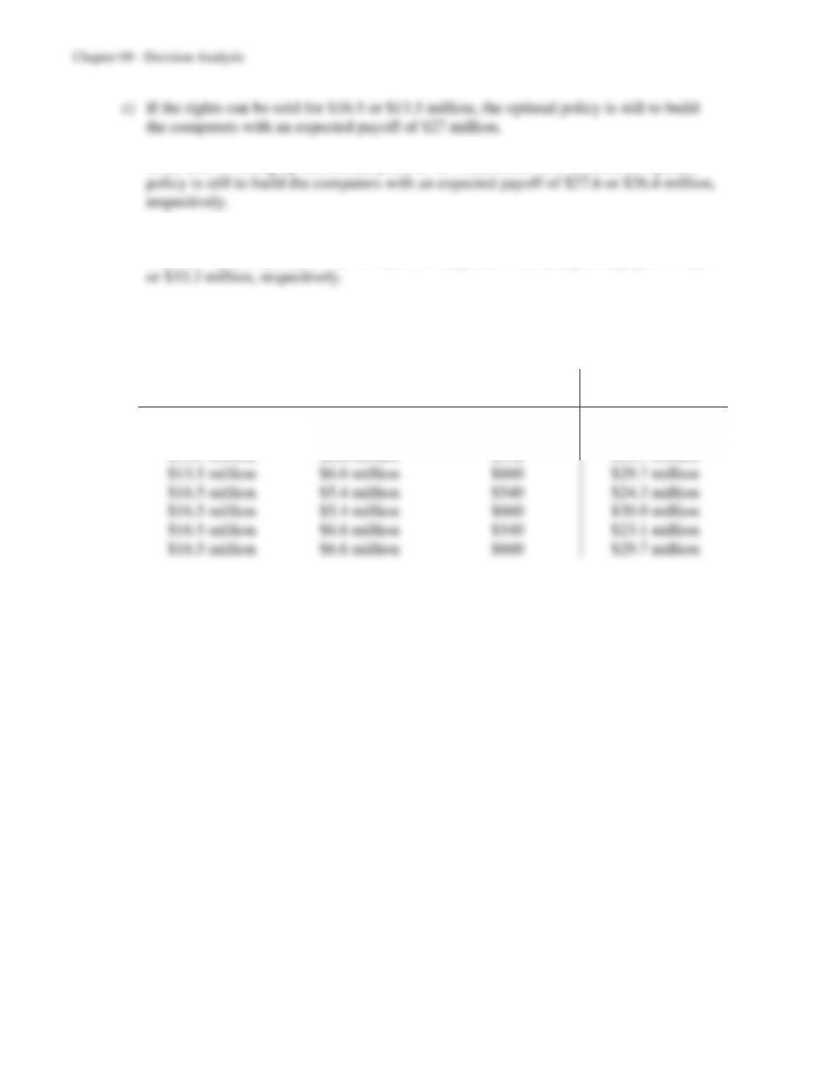
If the cost of setting up the assembly line is $5.4 million or $6.6 million, the optimal
If the difference between the selling price and variable cost of each computer is $540 or
$660, the optimal policy is still to build the computers with an expected payoff of $23.7
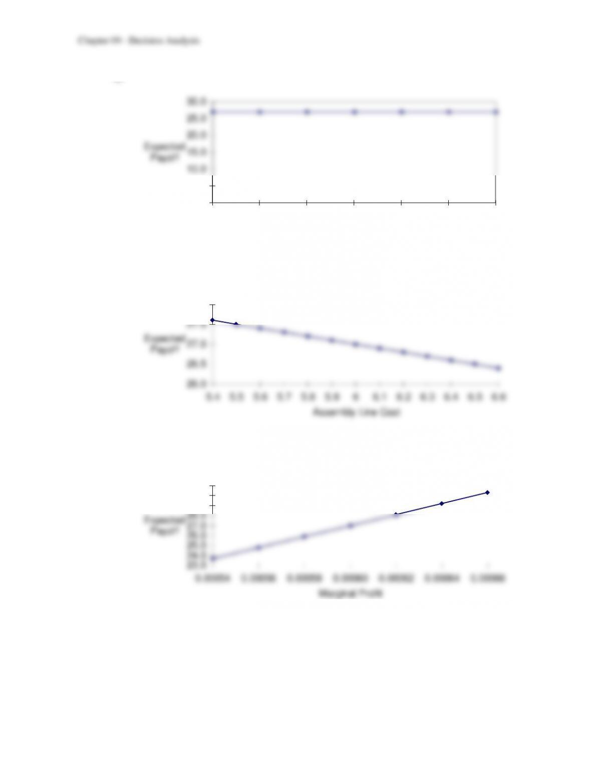
For each combination of financial data, the expected payoff is as shown below. In all
cases, the optimal policy is to build the computers (without market research).
Sell Rights
Cost of
Assembly Line
Selling Price –
Variable Cost
Expected
Payoff
$13.5 million
$5.4 million
$540
$24.3 million
$13.5 million
$5.4 million
$660
$30.9 million
$13.5 million
$6.6 million
$540
$23.1 million
$13.5 million
$6.6 million
$660
$29.7 million
$16.5 million
$5.4 million
$540
$24.3 million
$16.5 million
$5.4 million
$660
$30.9 million
$16.5 million
$6.6 million
$540
$23.1 million
$16.5 million
$6.6 million
$660
$29.7 million
9-51
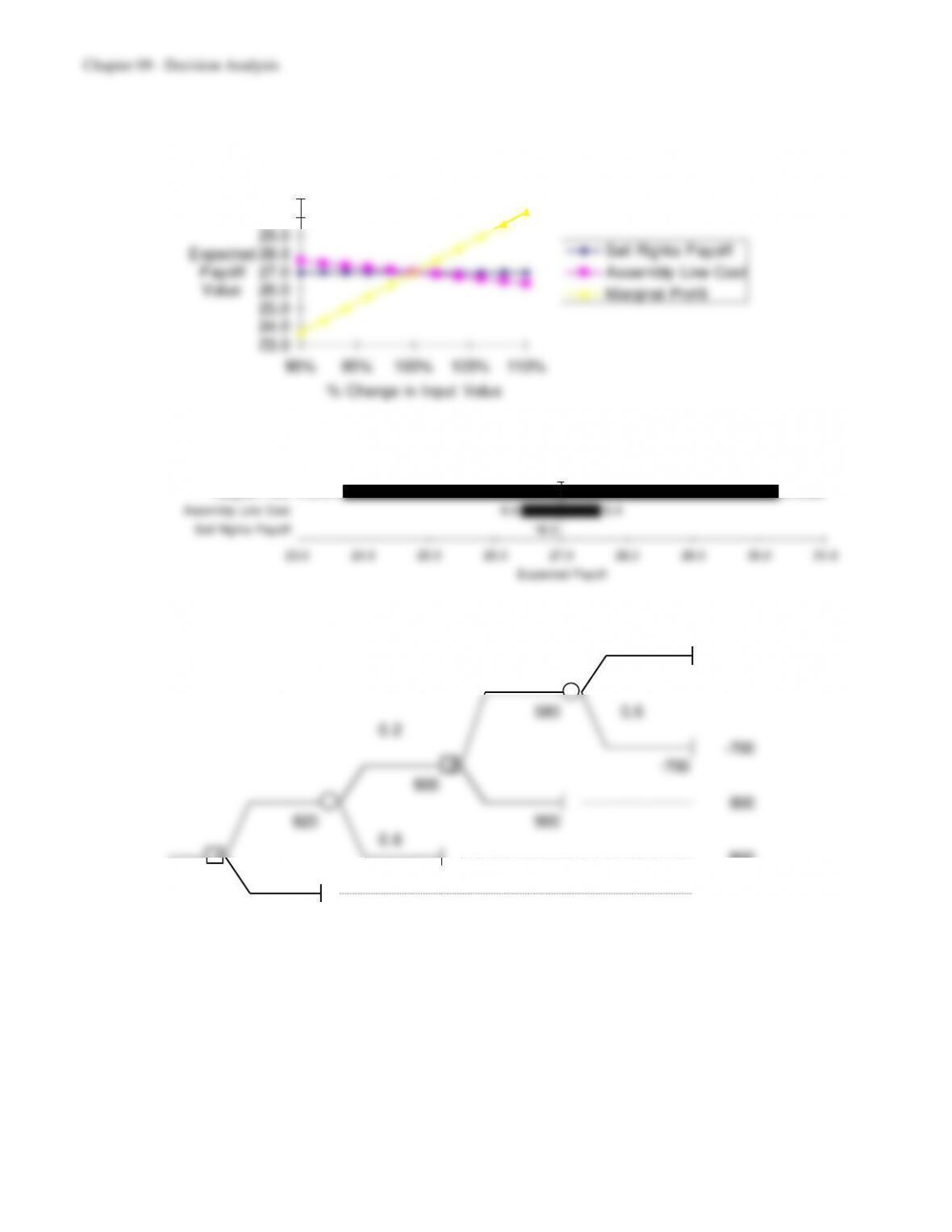
d)
0.0
5.0
10.0
15.0
20.0
25.0
30.0
13.5 14 14.5 15 15.5 16 16.5
Sell Rights Payoff
Expected
Payoff
Sensit – Sensitivity Analysis – Plo
26.0
26.5
27.0
27.5
28.0
5.4 5.5 5.6 5.7 5.8 5.9 6 6.1 6.2 6.3 6.4 6.5 6.6
Assembly Line Cost
Expected
Payoff
Sensit – Sensitivity Analysis – Plo
23.0
24.0
25.0
26.0
27.0
28.0
29.0
30.0
31.0
0.00054 0.00056 0.00058 0.00060 0.00062 0.00064 0.00066
Marginal Profit
Expected
Payoff
9-52
e)
Sensit – Sensitivity Analysis – Spide
23.0
24.0
25.0
26.0
27.0
28.0
29.0
30.0
31.0
90% 95% 100% 105% 110%
% Change in Input Value
Expected
Payoff
Value
Sell Rights Payoff
Assembly Line Cost
Marginal Profit
Sensit – Sensitivity Analysis – Tornad
13.5
5.4
0.00054
16.5
6.6
0.00066
23.0 24.0 25.0 26.0 27.0 28.0 29.0 30.0 31.0
Marginal Profit
Assembly Line Cost
Sell Rights Payoff
Expected Payoff
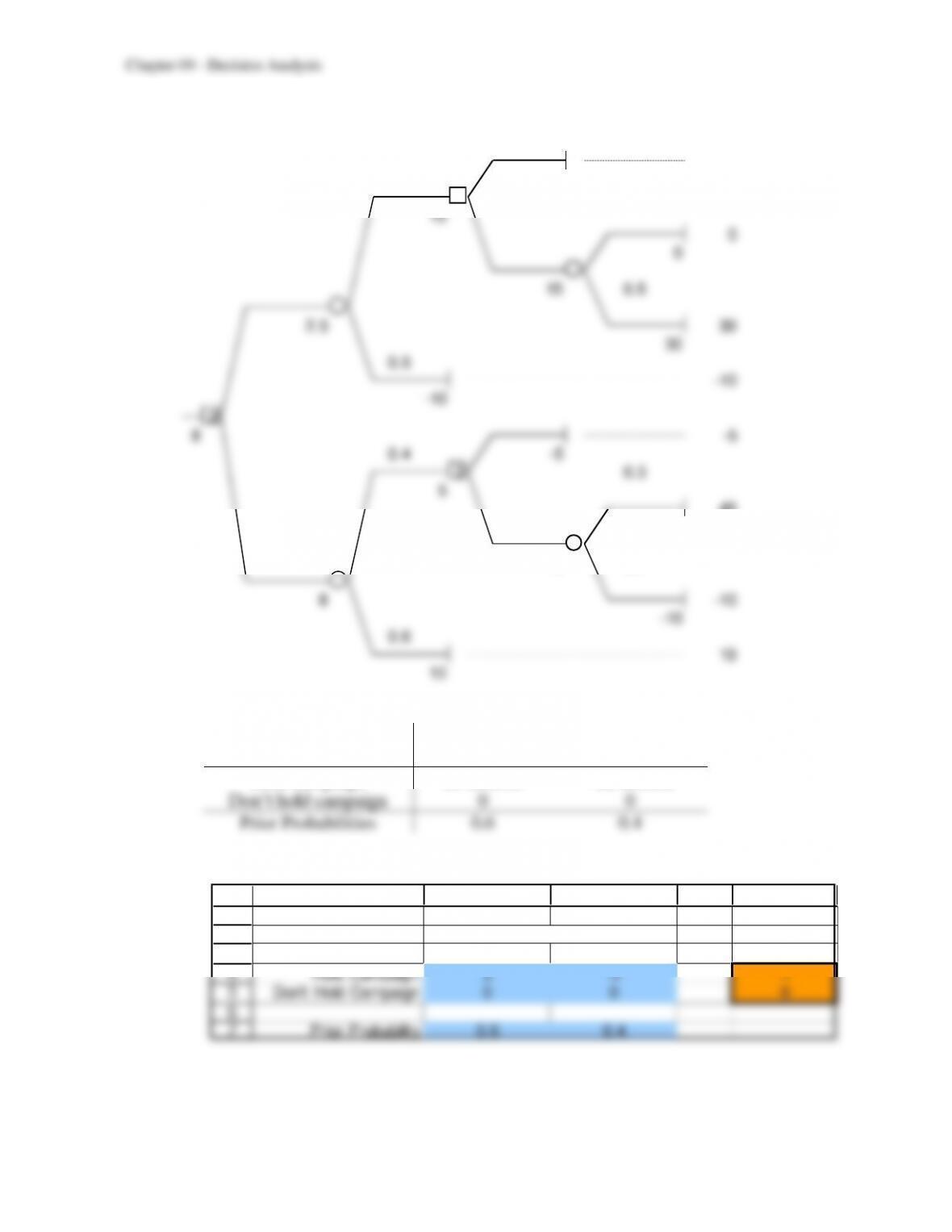
9.25 a and b)
0.4
2500
2500
580 0.6
0.2
-700
2 -700
900
900
820 900
0.8
1 800
820 800
750
750
9-53
9.26
10
0.5 10
2 0.5
15
0
0
15 0.5
2.5 30
30
0.5
–10
–10
2
8-5
0.4 -5
2 0.3
5
40
40
5 0.7
8 –10
–10
0.6
10
10
9.27 a)
State of Nature
Alternative
Winning Season
Losing Season
Hold campaign
$3 million
–$2 million
Don’t hold campaign
0
0
Prior Probabilities
0.6
0.4
b) Choosing to hold the campaign maximizes the expected payoff ($1 million).
1
2
3
4
5
6
7
A B C D E
Payoff Table ($millions) Expected
Payoff
Alternative Winning Season Losing Season ($millions)
Hold Campaign 3 -2 1
Don’t Hold Campaign 0 0 0
Prior Probability 0.6 0.4
State of Nature
c) With perfect information, Leland University should hold the campaign if they will have
a winning season and don’t hold the campaign if they will have a losing season.
d)
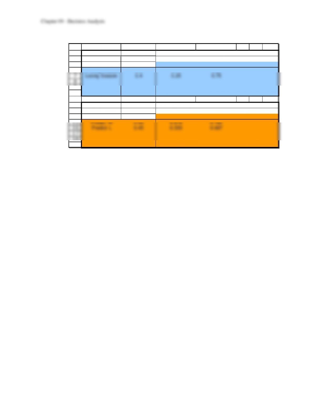
Prior
Probab ilities
P (state)
Conditional
Probab ilities
P(finding | state)
Jo int
Probab ilities
P(state and finding)
Pos terior
Probab ilities
P(state | finding
0.6
W in
Los e
0.4
win, given win
lose, given win
0.75
0.25
win, given lo se
lose, given lose
0.25
0.75
win and win
win and los e
0.45
0.15
lose an d win
lose an d lose
0.1
0.3
win. given win
win, given lo se
lose, given win
lose, given lose
0.818
0.333
0.667
0.182
9-55
e)
3
4
5
6
7
8
9
10
11
12
13
14
15
16
17
18
19
B C D E F G H
Data:
State of Prior
Nature Probability Predict W Predict L
Winning Season 0.6 0.75 0.25
Losing Season 0.4 0.25 0.75
Po sterio r
Pro bab il i ti es:
Finding P(Finding) Winning Season Losing Season
Predict W 0.55 0.818 0.182
Predict L 0.45 0.333 0.667
P(State | Finding)
State of Nature
P(Finding | State)
Finding
f & g) Leland University should hire William. If he predicts a winning season then they
should hold the campaign, if he predicts a losing season then they should not hold the
9-57
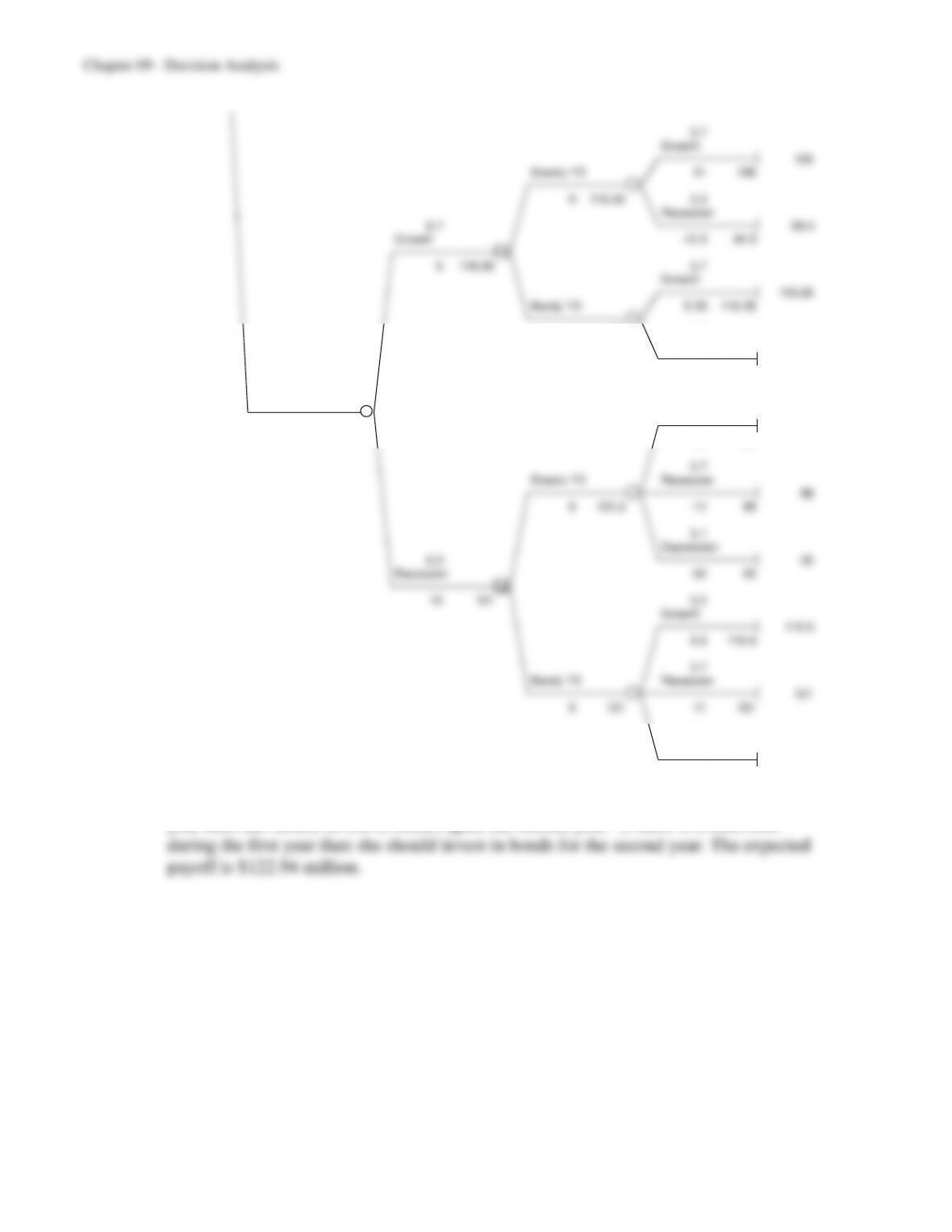
9.28 a & b) (Note: this decision tree continues on the next page.)
0.7
Growth
144
Stocks Y2 24 144
0 133.2 0.3
Recession
0.7 108
Growth -12 108
1
20 133.2 0.7
Growth
126
Bonds Y2 6 126
0 127.8 0.3
Recession
132
12 132
Stocks Y1 0.2
Growth
100 122.94 108
18 108
0.7
Stocks Y2 Recession
81
0 82.8 -9 81
0.1
Depression
0.3 45
Recession -45 45
2
-10 99 0.2
Growth
94.5
4.5 94.5
0.7
Bonds Y2 Recession
99
099 999
0.1
1 Depression
122.94 108
18 108
9-58
0.7
Growth
126
Stocks Y2 21 126
0 116.55 0.3
Recession
0.7 94.5
Growth -10.5 94.5
1
5 116.55 0.7
Growth
110.25
Bonds Y2 5.25 110.25
0 111.825 0.3
Recession
115.5
10.5 115.5
Bonds Y1 0.2
Growth
100 117.885 132
22 132
0.7
Stocks Y2 Recession
99
0 101.2 -11 99
0.1
Depression
0.3 55
Recession -55 55
2
10 121 0.2
Growth
115.5
5.5 115.5
0.7
Bonds Y2 Recession
121
0 121 11 121
0.1
Depression
132
22 132
The comptroller should invest in stocks the first year. If there is growth during the first
year then she should invest in stocks again the second year. If there is a recession
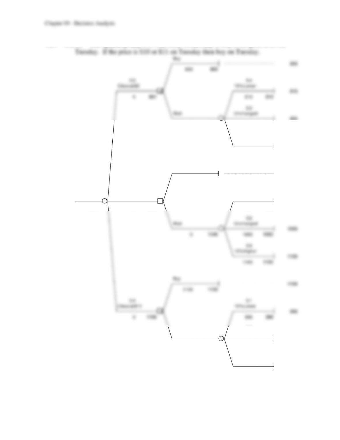
9.29 a & b) The optimal policy is to wait until Wednesday to buy if the price is $9 on
9-60
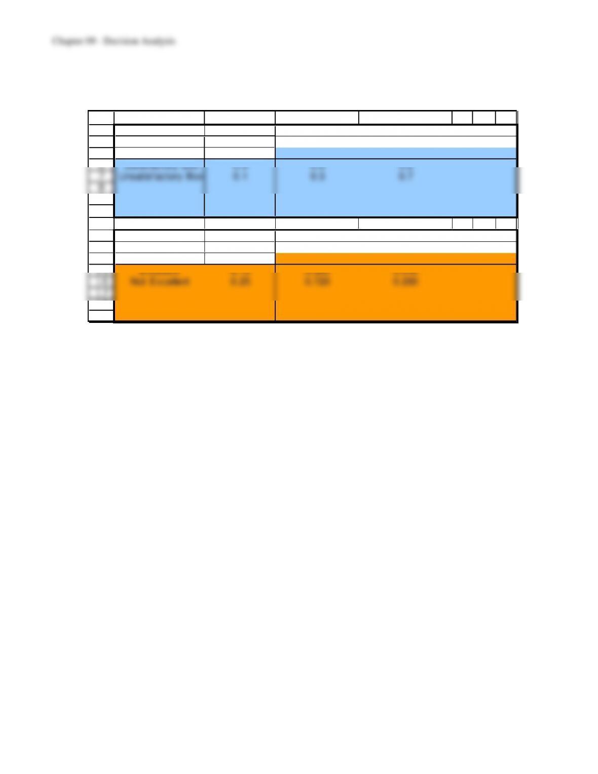
9.30 The optimal policy is to sample the fruit and buy if it is excellent and reject if it is
unsatisfactory.
3
4
5
6
7
8
9
10
11
12
13
14
15
16
17
18
19
B C D E F G H
Data:
State of Prior
Nature Probability Excellent Not Excellent
Satisfactory Box 0.9 0.8 0.2
Unsatisfactory Box 0.1 0.3 0.7
Po sterio r
Prob ab il iti es:
Finding P(Finding) Satisfactory Box Unsatisfactory Box
Excellent 0.75 0.960 0.040
Not Excellent 0.25 0.720 0.280
P(State | Finding)
State of Nature
P(Finding | State)
Finding