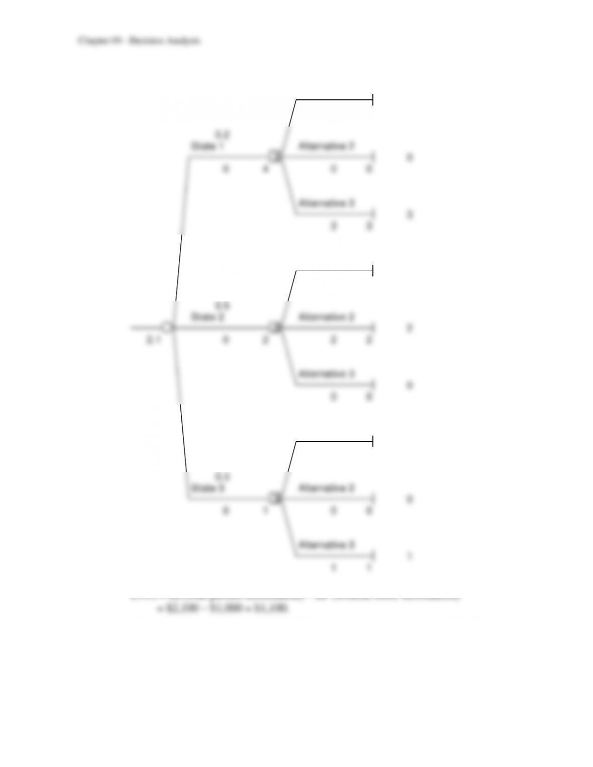
9-21
c)
Alternative 1
4
4 4
0.2
State 1 Alternative 2
1 0
0 4 0 0
Alternative 3
3
3 3
Alternative 1
0
0 0
0.5
State 2 Alternative 2
2 2
2.1 0 2 2 2
Alternative 3
0
0 0
Alternative 1
0
0 0
0.3
State 3 Alternative 2
3 0
0 1 0 0
Alternative 3
1
1 1
d) Since the information will cost $1,000 and the value is no more than $1,100, it might be
worthwhile to spend the money.
9-22
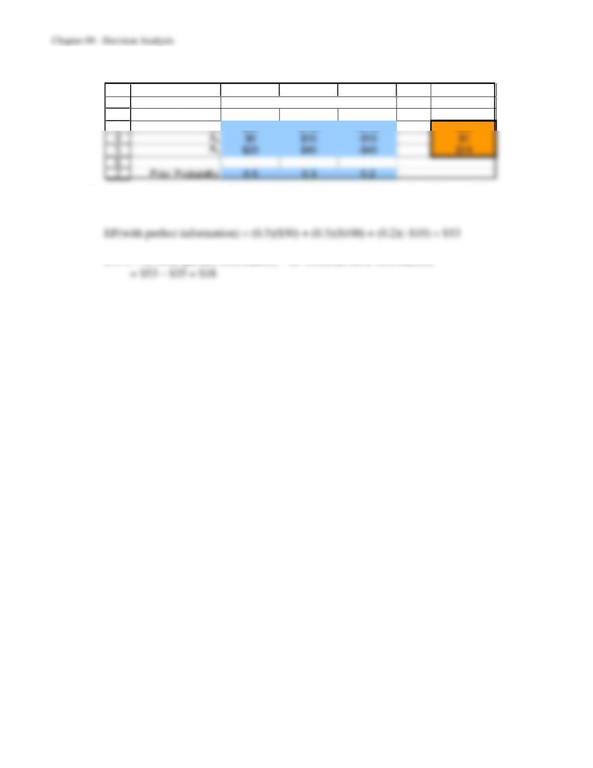
9.12 a) Alternative A1 has the highest expected payoff of $35.
1
2
3
4
5
6
7
A B C D E F
Payoff Table State of Nature Expected
Alternative
S1S2S3Payoff
A1$50 $100 -$100 $35
A2$0 $10 –$10 $1
A3$20 $40 -$40 $14
Prior Probability 0.5 0.3 0.2
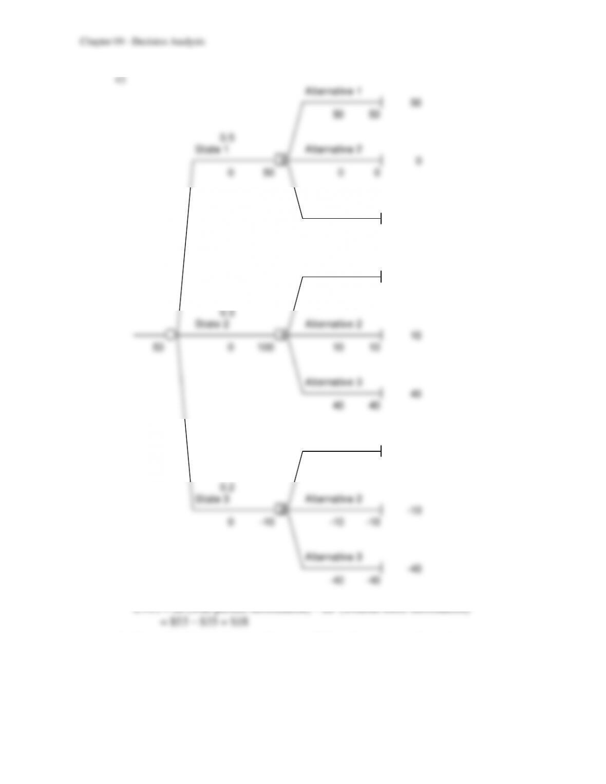
b) With perfect information, choose A1 for when the state is S1, A1 when the state is S2, and
A2 when the state is S3.
EVPI = EP(with perfect information) – EP (without more information)
9-23
Alternative 1
50
50 50
0.5
State 1 Alternative 2
1 0
050 0 0
Alternative 3
20
20 20
Alternative 1
100
100 100
0.3
State 2 Alternative 2
110
53 0 100 10 10
Alternative 3
40
40 40
Alternative 1
-100
-100 -100
0.2
State 3 Alternative 2
2 -10
0 -10 -10 -10
Alternative 3
-40
-40 -40
d) Betsy should consider spending up to $18 to obtain more information.
9-24
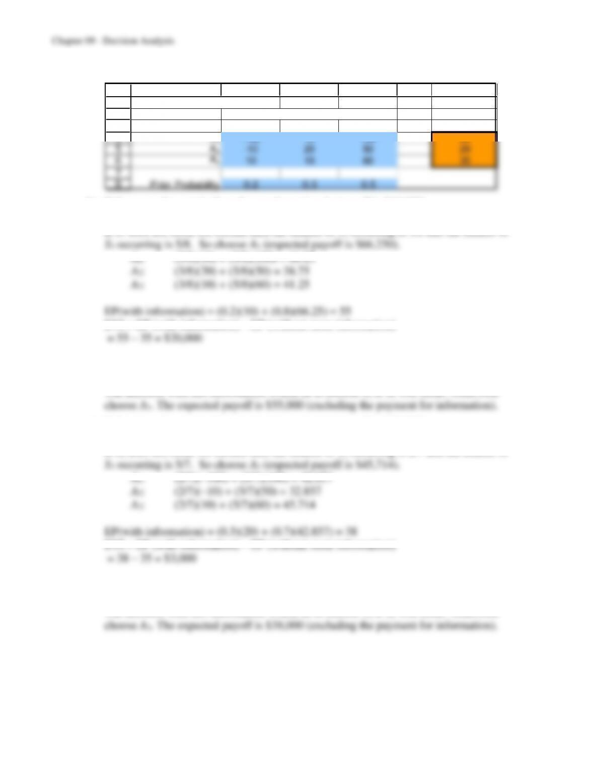
9.13 a) Alternative A3 has the highest expected payoff of $35,000.
1
2
3
4
5
6
7
8
A B C D E F
Payoff Table ($thousands) Expected
State of Nature Payoff
Alternative
S1S2S3($thousands)
A1-100 10 100 33
A2-10 20 50 29
A310 10 60 35
Prior Probability 0.2 0.3 0.5
b) If S1 occurs for certain then choose alternative A3 (payoff is $10,000).
If S1 does not occur for certain then the chance of S2 occurring is 3/8 and the chance of
EVI = EP (with information) – EP (without more information)
The maximum amount you should pay for the information is $20,000.
The decision with this information would be to choose A3 if S1 will occur. Otherwise
c) If S2 occurs for certain then choose alternative A2 (payoff is $20,000).
If S2 does not occur for certain then the chance of S1 occurring is 2/7 and the chance of
The maximum amount you should pay for the information is $3,000.
The decision with this information would be to choose A2 if S2 will occur. Otherwise
9-25
If S3 does not occur for certain then the chance of S1 occurring is 2/5 and the chance of
S2 occurring is 3/5. So choose A3 (expected payoff is $10,000).
A1: (2/5)(–100) + (3/5)(10) = –34
EP(with information) = (0.5)(100) + (0.5)(10) = 55
The maximum amount you should pay for the information is $20,000.
The decision with this information would be to choose A1 if S3 will occur. Otherwise
choose A3. The expected payoff is $55,000 (excluding the payment for information).
e) With perfect information, choose A3 for when the state is S1, A2 when the state is S2, and
A1 when the state is S3.
A maximum of $23,000 should be paid for the information. With perfect information,
choose A3 for when the state is S1, A2 when the state is S2, and A1 when the state is S3.
9-26
9.14 a)
b)
3
4
5
6
7
8
9
10
11
12
13
14
15
16
17
18
19
B C D E F G H
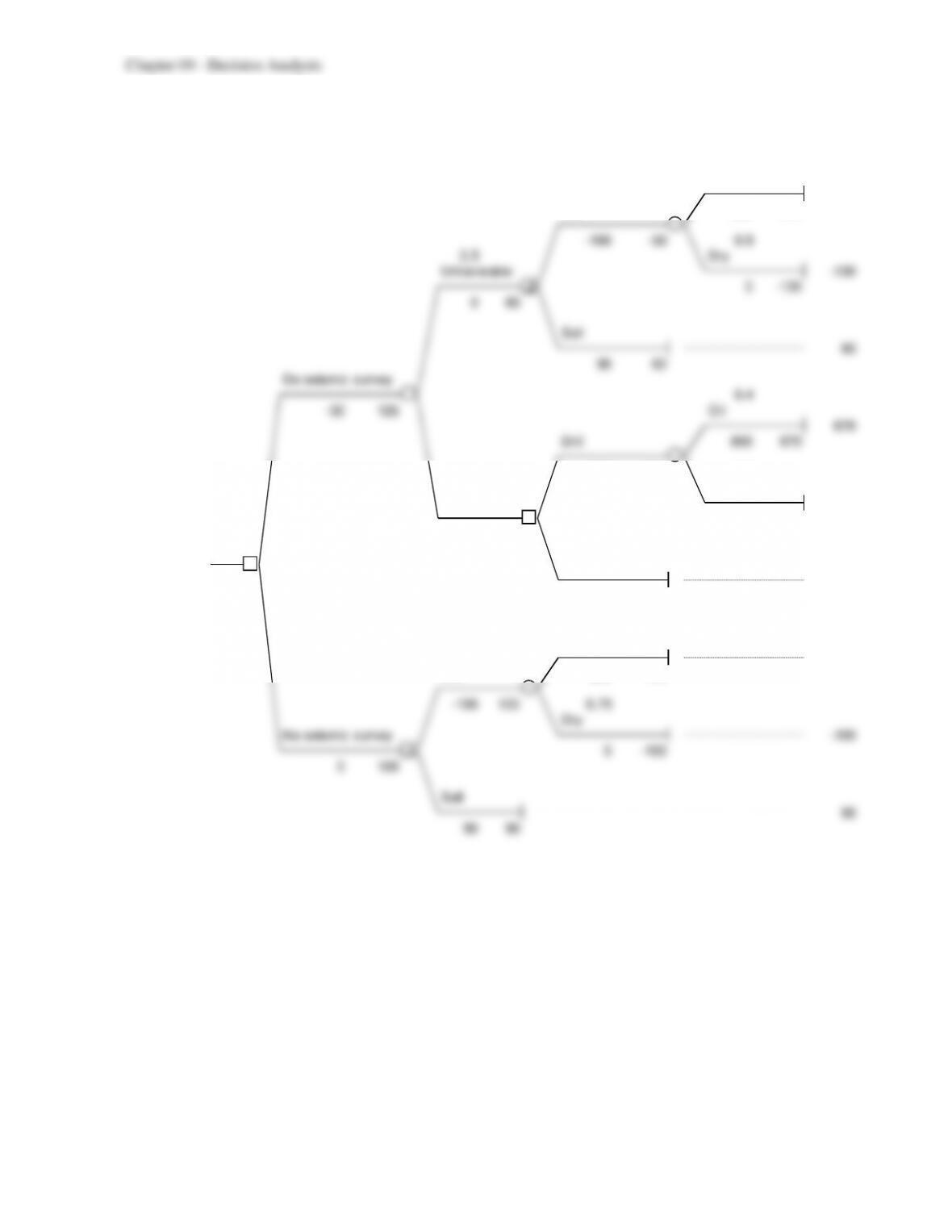
Data:
State of Prior
Nature Probability FSS USS
Oil 0.25 0.8 0.2
Dry 0.75 0.4 0.6
Posterior
Prob abilities:
Finding P(Finding) Oil Dry
FSS 0.5 0.4 0.6
USS 0.5 0.1 0.9
P(State | Finding)
State of Nature
P(Finding | State)
Finding
9-27
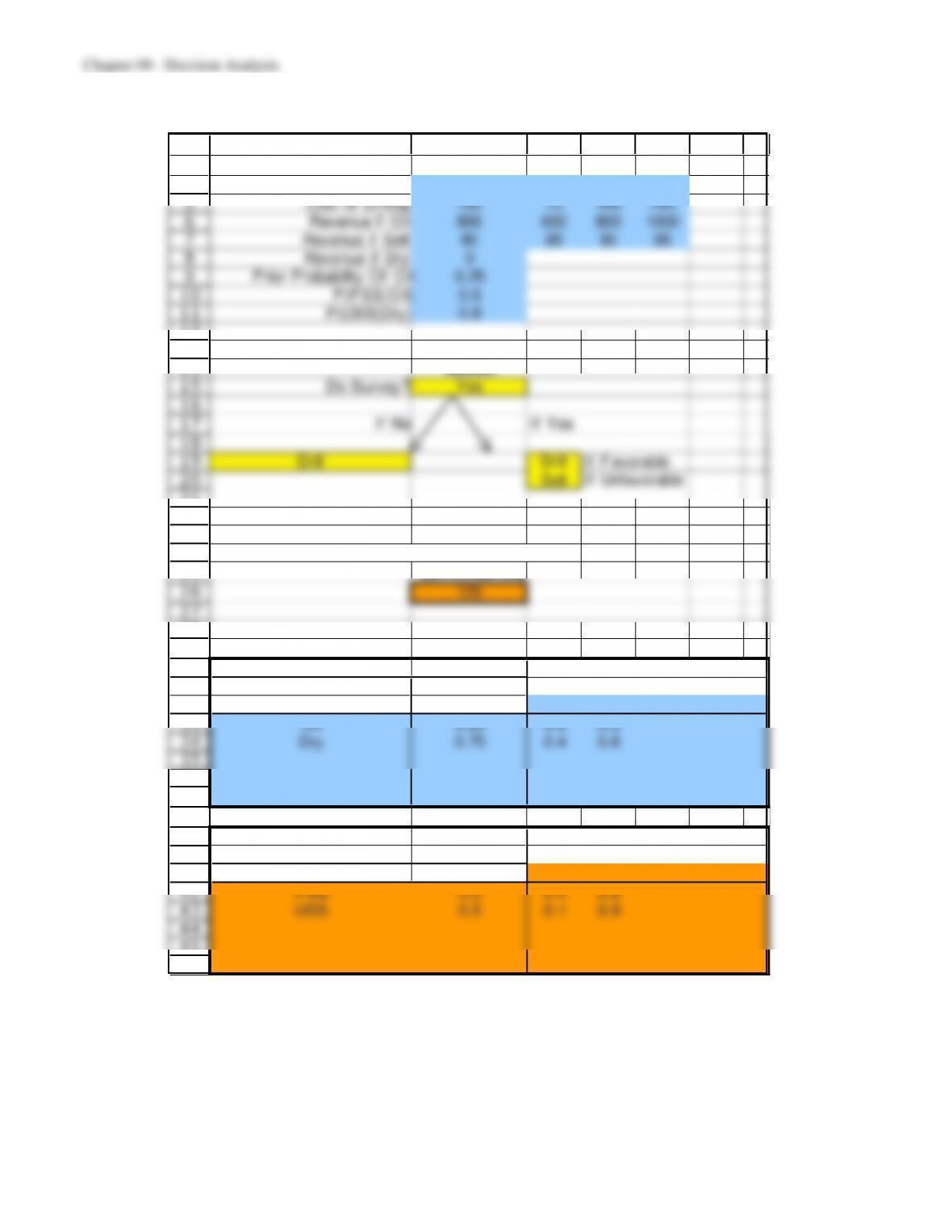
c & d) The optimal policy is to do a seismic survey and sell if it is unfavorable or drill if
it is favorable.
0.1
Oil
670
Drill 800 670
-100 -50 0.9
0.5 Dry
Unfavorable -130
2 0 -130
060
Sell
60
90 60
Do seismic survey
0.4
-30 125 Oil
670
Drill 800 670
-100 190 0.6
0.5 Dry
Favorable -130
1 0 -130
0 190
1 Sell
125 60
90 60
0.25
Oil
700
Drill 800 700
-100 100 0.75
Dry
No seismic survey -100
1 0 -100
0 100
Sell
90
90 90
9-28
9.15 a)
3
4
5
6
7
8
9
10
11
12
13
14
15
16
17
18
19
20
21
22
23
24
25
26
27
28
29
30
31
32
33
34
35
36
37
38
39
40
41
42
43
44
45
46
U V W X Y Z AA
Data Low Base High
Cost of Survey 30 28 30 32
Cost of Drilling 100 75 100 140
Revenue if Oil 800 600 800 1000
Revenue if Sell 90 85 90 95
Revenue if Dry 0
Prior Probability Of Oil 0.25
P(FSS|Oil) 0.6
P(USS|Dry) 0.8
Action
Do Survey? Yes
If No If Yes
Drill Drill If Favorable
Sell If Unfavorable
Expected Payoff
($thousands)
125
Data:
State of Prior
Nature Probability FSS USS
Oil 0.25 0.8 0.2
Dry 0.75 0.4 0.6
Posterior
Probabilities:
Finding P(Finding) Oil Dry
FSS 0.5 0.4 0.6
USS 0.5 0.1 0.9
P(State | Finding)
Finding
State of Nature
P(Finding | State)
9-29
b)
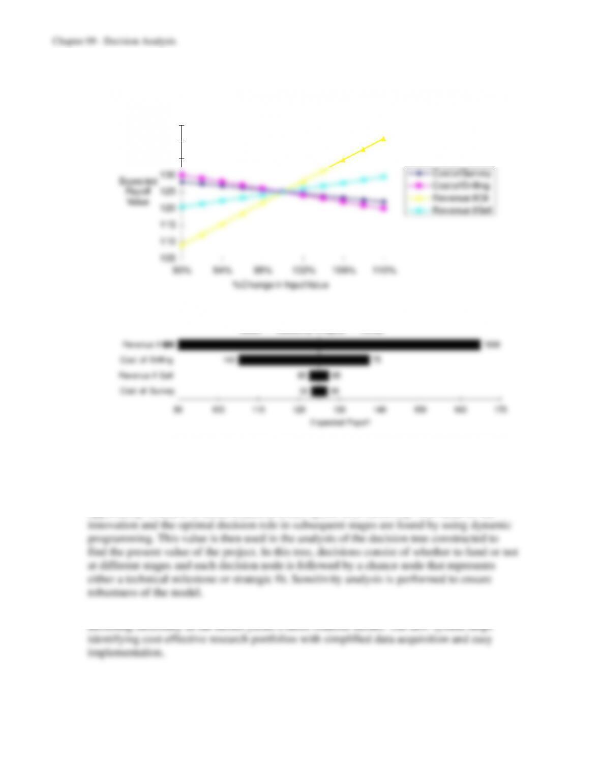
Sensit – Sensitivity Analysis – Plo
100
110
120
130
140
150
160
0 0.1 0.2 0.3 0.4 0.5 0.6 0.7 0.8 0.9 1
P(FSS|Oil)
Expected
Payoff
Sensit – Sensitivity Analysis – Plo
100
110
120
130
140
150
160
170
180
190
0 0.1 0.2 0.3 0.4 0.5 0.6 0.7 0.8 0.9 1
P(FSS|Dry)
Expected
Payoff
9-30
c)
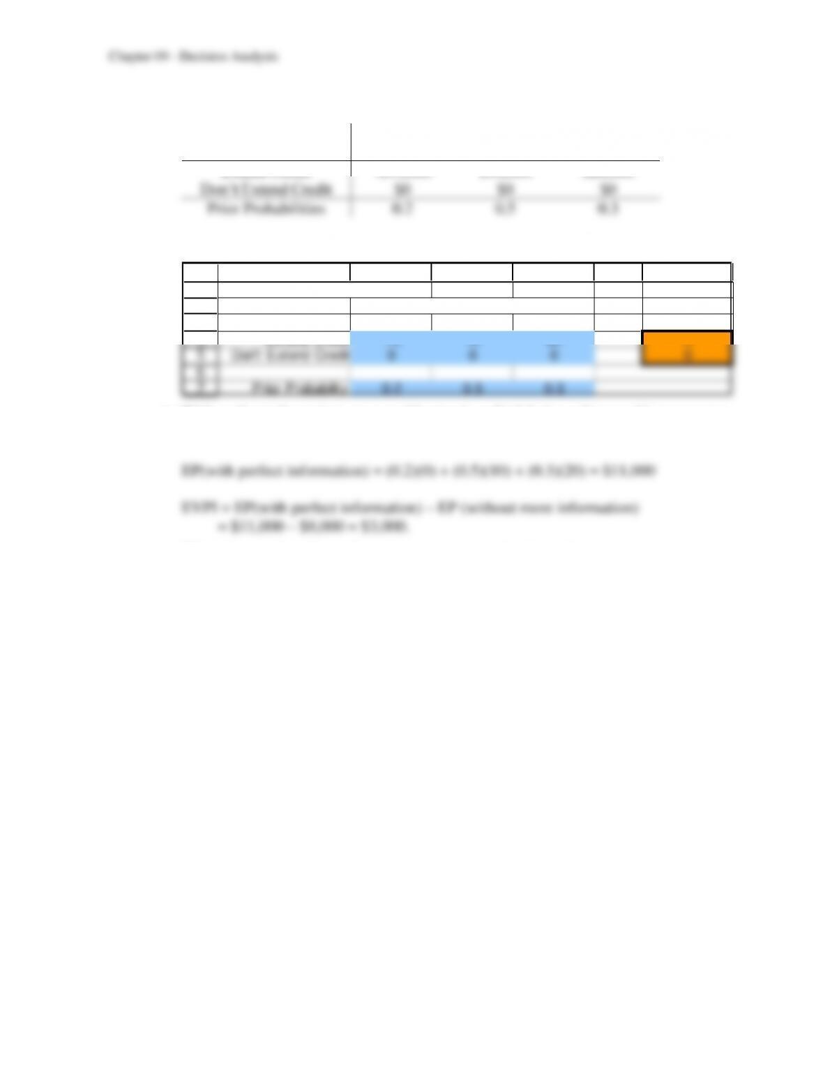
Sensit – Sensitivity Analysis – Spider
105
110
115
120
125
130
135
140
145
90% 94% 98% 102% 106% 110%
% Change in Input Value
Expected
Payoff
Value
Cost of Survey
Cost of Drilling
Revenue if Oil
Revenue if Sell
Sensit – Sensitivity Analysis – Tornad
28
85
75
600
32
95
140
1000
90 100 110 120 130 140 150 160 170
Revenue if Oil
Cost of Drilling
Revenue if Sell
Cost of Survey
Expected Payoff
9.16 Driven by “the pressure to reduce costs and deliver high-impact technology quickly while
justifying investments” [p. 57], Westinghouse initiated this study to evaluate R and D
efforts effectively. At any point in time, the firm chooses between launching, delaying and
abandoning an innovation. When the launch is delayed, there is a chance of losing the
opportunity. R and D is hence treated as a call option with flexibility. The value of the
As a result of this study, explicit decision rules for funding R and D projects are obtained.
Including flexibility in the model yields a more realistic model. The new system helps
9-31
9.17 a)
State of Nature
Alternative
Poor Risk
Average Risk
Good Risk
Extend Credit
-$15,000
$10,000
$20,000
Don’t Extend Credit
$0
$0
$0
Prior Probabilities
0.2
0.5
0.3
b) Extending credit maximizes the expected payoff ($8,000).
1
2
3
4
5
6
7
A B C D E F
Payoff Table ($thousands) Expected
State of Nature (Credit Record) Payoff
Alternative Poor Average Good ($thousands)
Extend Credit –15 10 20 8
Don’t Extend Credit 0 0 0 0
Prior Probability 0.2 0.5 0.3
c) With perfect information, you would extend credit if their credit record is average or
good, and don’t extend credit if their credit record is poor.
This indicates that the credit-rating organization should not be used.
9-32
0.06
0.12
0.1667
0.2667
0.3
GS and PF
GS, given PF
PF, g iven GS
0.2
0.4
9-33
e)
1
2
3
4
5
6
7
8
9
10
11
12
13
14
15
16
17
18
19
A B C D E F G H
Template for Posterior Probabilities
Data:
State of Prior
Nature Probability Poor Average Good
Poor 0.2 0.5 0.4 0.1
Average 0.5 0.4 0.5 0.1
Good 0.3 0.2 0.4 0.4
Posterior
Probabilities:
Finding P(Finding) Poor Average Good
Poor 0.36 0.278 0.556 0.167
Average 0.45 0.178 0.556 0.267
Good 0.19 0.105 0.263 0.632
P(State | F inding)
State of Nature
P(Finding | State)
Finding
9-34

Chapter 09 – Decision Analysis
9-35
9-36
h) EVSI = Value with credit rating (ignoring cost) – expected value without
The sample information provides no value. This is clear because the same decision is
made regardless of the findings of the credit report. (Note there is some rounding error.
Without the rounding error, the expected payoff with the credit rating is 3000 rather
than 2992.15.)
9.18 a) Alternative A1 maximizes the expected payoff ($100).
1
2
3
4
5
6
A B C D E
Payoff T able Expected
Alternative
S1S2Payoff
A1$400 –$100 $100
A2$0 $100 $60
Prior Probability 0.4 0.6
State of Nature
b)
Alternative 1
0.4 400
State 1 400 400
1
0 400
Alternative 2
0
0 0
220
Alternative 1
0.6 –100
State 2 –100 –100
2
0 100
Alternative 2
100
100 100
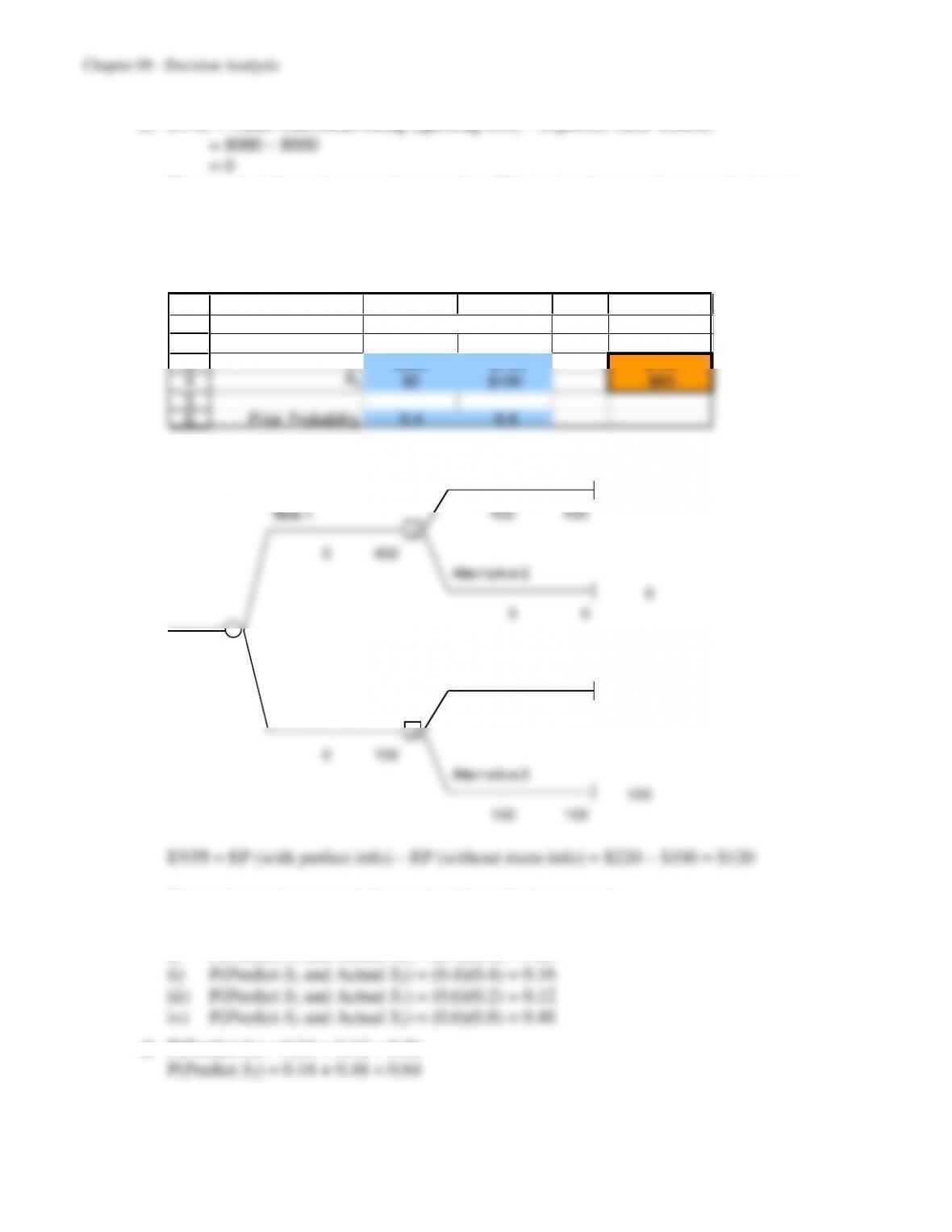
EVPI = EP (with perfect info) – EP (without more info) = $220 – $100 = $120
This indicates that it might be worthwhile to do the research.
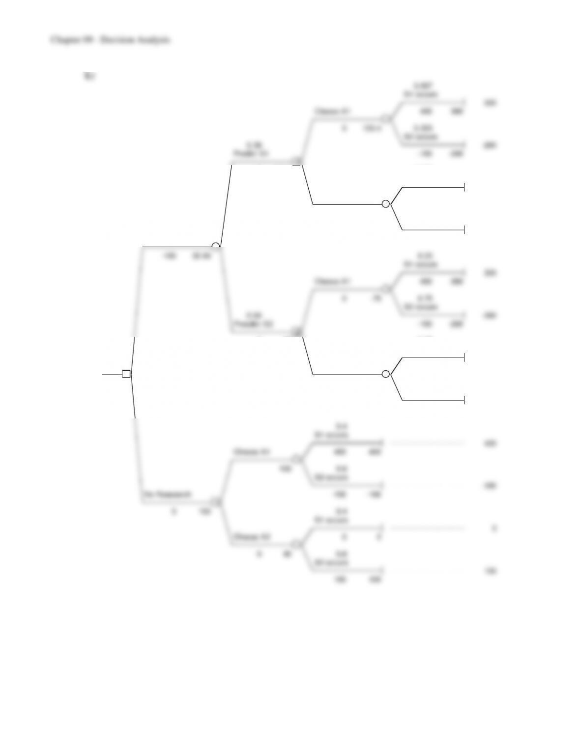
d) P(Predict S1) = 0.24 + 0.12 = 0.36
9-37
e) P(state | finding) = P(state and finding) / P(finding)
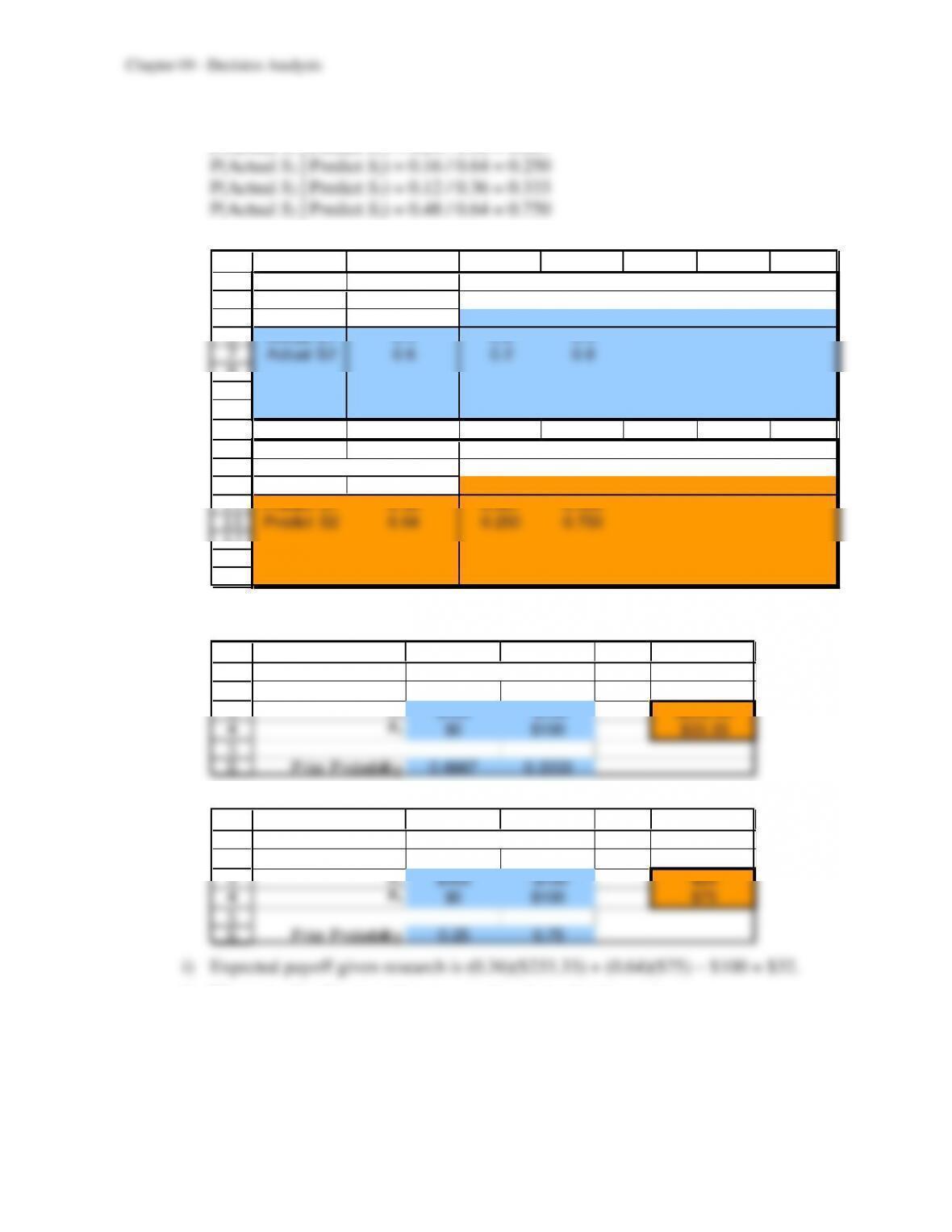
P(Actual S1 | Predict S1) = 0.24 / 0.36 = 0.667
f)
3
4
5
6
7
8
9
10
11
12
13
14
15
16
17
18
19
B C D E F G H
Data:
State of Prior
Nature Probability Predict S1 Predict S2
Actual S1 0.4 0.6 0.4
Actual S2 0.6 0.2 0.8
Posterior
Probabilities:
Finding P(Finding) Actual S1 Actual S2
Predict S1 0.36 0.667 0.333
Predict S2 0.64 0.250 0.750
P(State | Finding)
State of Nature
P(Finding | State)
Finding
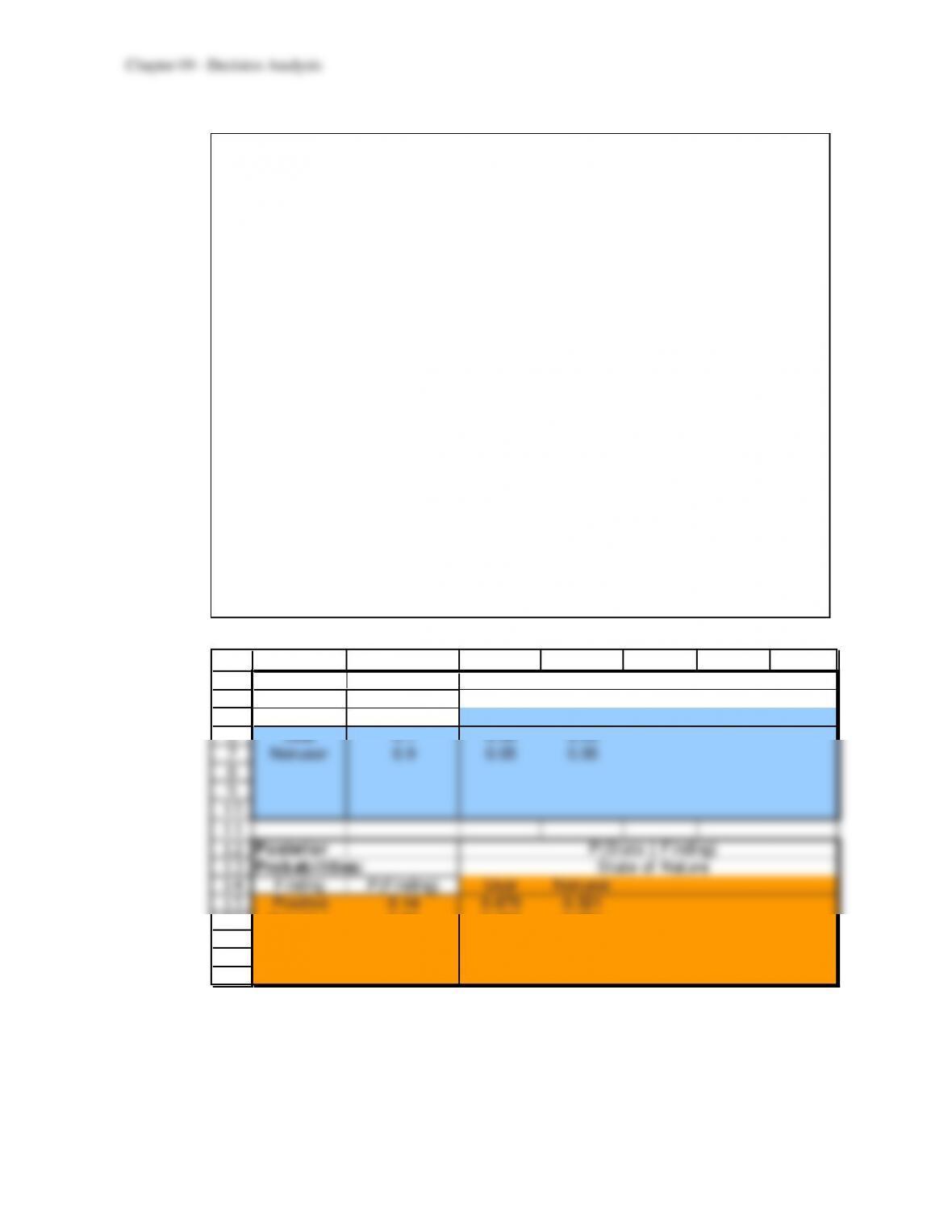
g) If S1 is predicted, then choosing alternative A1 maximizes the expected payoff
($233.33).
1
2
3
4
5
6
A B C D E
Payoff T able Expected
Alternative
S1S2Payoff
A1$400 –$100 $233.33
A1$0 $100 $33.33
Prior Probability 0.6667 0.3333
State of Nature
h) If S2 is predicted, then choosing alternative A2 maximizes the expected payoff ($75).
1
2
3
4
5
6
A B C D E
Payoff T able Expected
Alternative
S1S2Payoff
A1$400 –$100 $25
A1$0 $100 $75
Prior Probability 0.25 0.75
State of Nature
j) The optimal policy is to do no research and simply choose A1.
9-39
9.19 a through d)
e)
3
4
5
6
7
8
9
10
11
12
13
14
15
16
17
18
19
B C D E F G H
Data:
State of Prior
Nature Probability Positive Negative
User 0.1 0.95 0.05
Nonuser 0.9 0.05 0.95
Posterior
Probabilities:
Finding P(Finding) User Nonuser
Positive 0.14 0.679 0.321
Negative 0.86 0.006 0.994
P(State | Finding)
State of Nature
P(Finding | State)
Finding
9-40
9.20 a)
State of Nature
Alternative
Successful
Unsuccessful
Develop new product
$1,500,000
–$1,800,000
Don’t develop new product
0
0
Prior Probabilities
0.667
0.333
b) Choosing to develop the product maximizes the expected payoff ($400,000).
1
2
3
4
5
6
7
A B C D E
Payoff Table ($millions) Expected
Payoff
Alternative Successful Unsuccessful ($millions)
Develop Product 1.5 -1.8 0.4
Don‘t Develop Product 0 0 0
Prior Probability 0.667 0.333
State of Nature
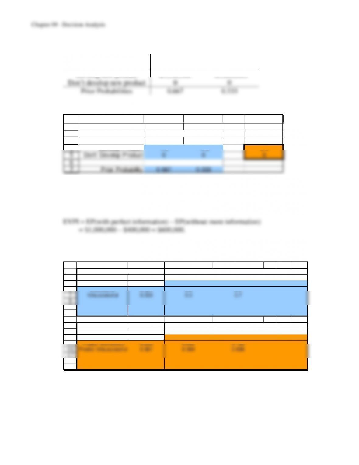
c) With perfect information, Telemore should develop the product if it would be
successful, and don’t if it will be unsuccessful.
EP(perfect information) = (0.667)(1.5) + (0.333)(0) = $1 million.
This indicates that consideration should be given to conducting the market survey.
d)
3
4
5
6
7
8
9
10
11
12
13
14
15
16
17
18
19
B C D E F G H
Data:
State of Prior
Nature Probability Predict Successful Predict Unsuccessful
Successful 0.667 0.8 0.2
Unsuccessful 0.333 0.3 0.7
Posterior
Probabilities:
Finding P(Finding) Successful Unsuccessful
Predict Successful 0.633 0.842 0.158
Predict Unsuccessful 0.367 0.364 0.636
P(State | Finding)
State of Nature
P(Finding | State)
Finding