Chapter 09 – Decision Analysis
Chapter 9 Decision Analysis
Review Questions
9.1-1 The decision alternatives are to drill for oil or to sell the land.
9.1-2 The consulting geologist believes that there is 1 chance in 4 of oil on the tract of land.
9.1-3 Max does not put much faith in the assessment.
9.1-4 A detailed seismic survey of the land could be done to obtain more information.
9.1-6 Prior probabilities are the estimated probabilities of the states of nature prior to obtaining
additional information through a test or survey.
9.2-1 The maximax criterion identifies the maximum payoff for each decision alternative and
chooses the decision alternative with the maximum of these maximum payoffs. The
maximax criterion is for the eternal optimist.
9.2-3 The maximin criterion identifies the minimum payoff for each decision alternative and
chooses the decision alternative with the maximum of these minimum payoffs. The
maximin criterion is for the total pessimist.
9.2-5 The maximum likelihood criterion focuses on the most likely state of nature, the one with
the largest prior probability.
9.2-6 Criticisms of the maximum likelihood criterion include: 1) this criterion chooses an
alternative without considering its payoffs for states of nature other than the most likely
one, 2) for alternatives that are not chosen, this criterion ignores their payoffs for states of
9.2-7 Bayes’ decision rule says to choose the alternative with the largest expected payoff.
9.2-8 The expected payoff is calculated by multiplying each payoff by the prior probability of the
corresponding state of nature and then summing these products.
9-3
9.6-6 P(finding) = sum of P(state and finding) for each state.
9.6-8 Bayes’ theorem is used to calculate posterior probabilities.
9.7-1 A decision tree provides a graphical display of the progression of decisions and random
events for a problem.
9.7-2 A decision needs to be made at a decision node.
9.7-4 The probabilities of random events and the payoffs need to be inserted before beginning
analysis.
9.7-5 When performing the analysis, start at the right side of the decision tree and move left one
column at a time.
9.7-7 For each decision node, compare the expected payoffs of its branches and choose the
alternative whose branch has the largest expected payoff.
9.8-1 Consolidate the data and results into one section of the spreadsheet.
9.8-2 Performing sensitivity analysis on a piece of data should require changing a value in only
one place on the spreadsheet.
9.8-3 A data table can consider changes in only one or two data cells.
9.8-4 One.
9.8-5 Yes. The spider graph can consider changes in many data cells at a time.
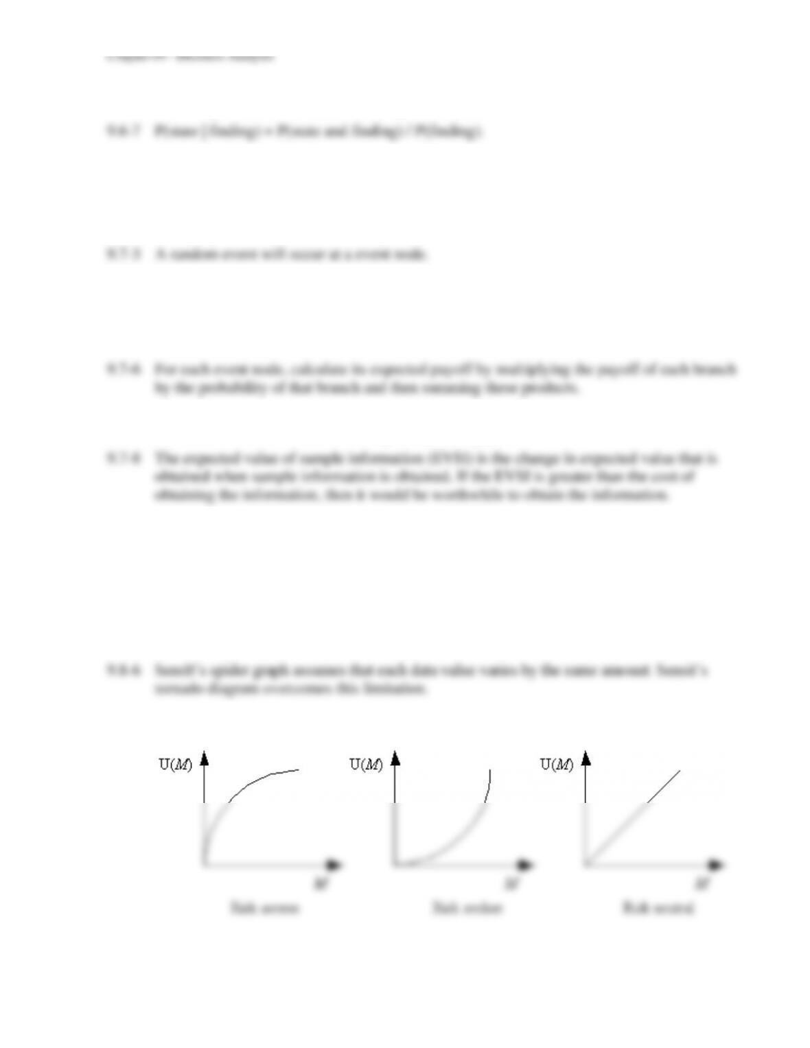
9.9-1 Utilities are intended to reflect the true value of an outcome to the decision-maker.
9.9-2
9-4
9.9-3 Under the assumptions of utility theory, the decision-maker’s utility function for money
has the property that the decision-maker is indifferent between two alternative courses of
action if the two alternatives have the same expected utility.
9.9-5 The point of indifference is the value of p where the decision-maker is indifferent between
the two hypothetical alternatives.
9.9-6 The value obtained to evaluate each node of the tree is the expected utility.
9.9-7 Max decided to do the seismic survey and to sell if the result is unfavorable or drill if the
result is favorable.
9.10-2 An influence diagram complements the decision tree for representing and analyzing
decision analysis problems.
Problems
9.1 a) Max(A1) = 6, Max(A2) = 4, Max(A3) = 8. Maximax = 8 with alternative A3.
9.2 a) Max(A1) = 30, Max(A2) = 31, Max(A3) = 22, Max(A4) = 29. Maximax = 31 with A2.
9.3 a)
State of Nature
Alternative
Sell 10
cases
Sell 11 cases
Sell 12
cases
Sell 13
cases
Buy 10 cases
$50
$50
$50
$50
Buy 11 cases
$47
$55
$55
$55
Buy 12 cases
$44
$52
$60
$60
Buy 13 cases
$41
$49
$57
$65
Prior
Probability
0.2
0.4
0.3
0.1
b) Max(Buy 10) = $50, Max(Buy 11) = $55, Max(Buy 12) = $60, Max(Buy 13) = $65.
Maximin = $50 with buying 10 cases.
9-5
e)
1
2
3
4
5
6
7
8
9
10
11
12
A B C D E F G H
Purchase Price $3
Selling Price $8
Payoff Table
Sell Sell Sell Sell Expected
Alternative 10 11 12 13 Payoff
Buy 10 $50 $50 $50 $50 $50.00
Buy 11 $47 $55 $55 $55 $53.40
Buy 12 $44 $52 $60 $60 $53.60
Buy 13 $41 $49 $57 $65 $51.40
Prior Probability 0.2 0.4 0.3 0.1
State of Nature
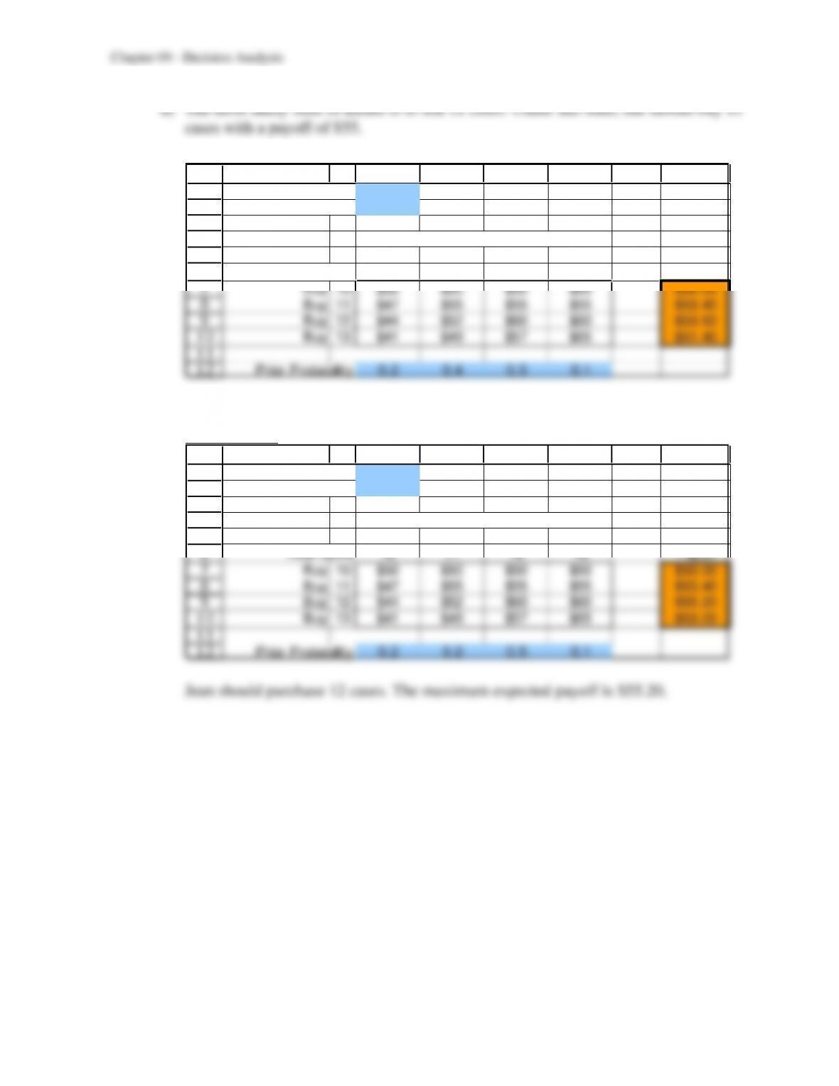
Jean should buy 12 cases. The maximum expected payoff is $53.60.
f) (i) 0.2 and 0.5
1
2
3
4
5
6
7
8
9
10
11
12
A B C D E F G H
Purchase Price $3
Selling Price $8
Payoff Table
Sell Sell Sell Sell Expected
Alternative 10 11 12 13 Payoff
Buy 10 $50 $50 $50 $50 $50.00
Buy 11 $47 $55 $55 $55 $53.40
Buy 12 $44 $52 $60 $60 $55.20
Buy 13 $41 $49 $57 $65 $53.00
Prior Probability 0.2 0.2 0.5 0.1
State of Nature
9-6
(ii) 0.3 and 0.4
1
2
3
4
5
6
7
8
9
10
11
12
A B C D E F G H
Purchase Price $3
Selling Price $8
Payoff Table
Sell Sell Sell Sell Expected
Alternative 10 11 12 13 Payoff
Buy 10 $50 $50 $50 $50 $50.00
Buy 11 $47 $55 $55 $55 $53.40
Buy 12 $44 $52 $60 $60 $54.40
Buy 13 $41 $49 $57 $65 $52.20
Prior Probability 0.2 0.3 0.4 0.1
State of Nature
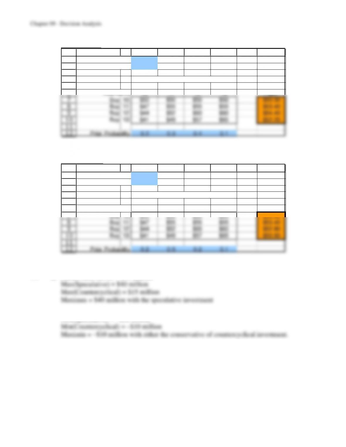
Jean should purchase 12 cases. The maximum expected payoff is $54.40.
(iii) 0.5 and 0.2
1
2
3
4
5
6
7
8
9
10
11
12
A B C D E F G H
Purchase Price $3
Selling Price $8
Payoff Table
Sell Sell Sell Sell Expected
Alternative 10 11 12 13 Payoff
Buy 10 $50 $50 $50 $50 $50.00
Buy 11 $47 $55 $55 $55 $53.40
Buy 12 $44 $52 $60 $60 $52.80
Buy 13 $41 $49 $57 $65 $50.60
Prior Probability 0.2 0.5 0.2 0.1
State of Nature
Jean should purchase 11 cases. The maximum expected payoff is $53.40.
9.4 a) Max(Conservative) = $30 million
b) Min(Conservative) = –$10 million
Min(Speculative) = –$30 million
c) The stable economy is the most likely state of nature.
The speculative investment has the maximum payoff for this state ($10 million).
9-7
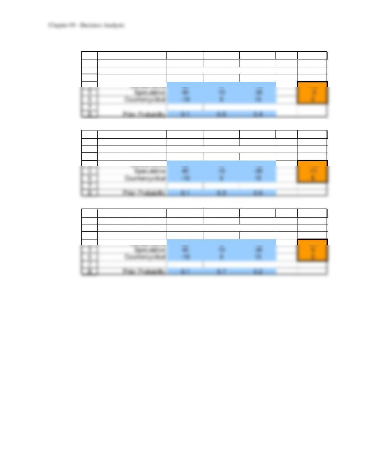
d) The countercyclical investment has the maximum expected payoff of $5 million.
1
2
3
4
5
6
7
8
A B C D E F
Payoff Table ($million) Expected
Alternative State of Nature (Economy) Payoff
(Investment) Improving Stable Worsening ($million)
Conservative 30 5 –10 1.5
Speculative 40 10 -30 -3
Countercyclical -10 0 15 5
Prior Probability 0.1 0.5 0.4
9.5 a) The countercyclical investment has the maximum expected payoff of $8 million.
1
2
3
4
5
6
7
8
A B C D E F
Payoff Table ($million) Expected
Alternative State of Nature (Economy) Payoff
(Investment) Improving Stable Worsening ($million)
Conservative 30 5 –10 -1.5
Speculative 40 10 -30 -11
Countercyclical -10 0 15 8
Prior Probability 0.1 0.3 0.6
b) The speculative investment has the maximum expected payoff of $5 million.
1
2
3
4
5
6
7
8
A B C D E F
Payoff Table ($million) Expected
Alternative State of Nature (Economy) Payoff
(Investment) Improving Stable Worsening ($million)
Conservative 30 5 –10 4.5
Speculative 40 10 -30 5
Countercyclical -10 0 15 2
Prior Probability 0.1 0.7 0.2
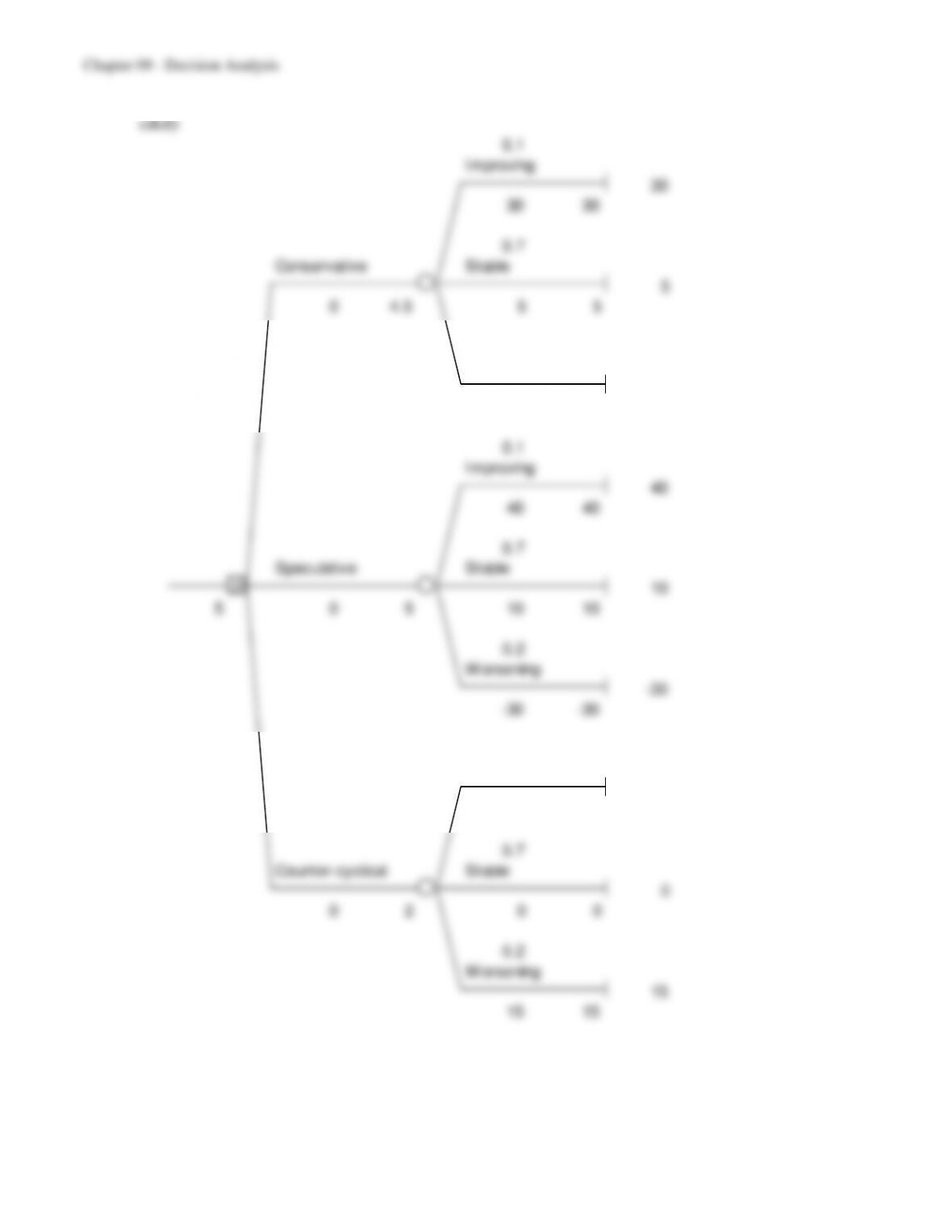
9-8
0.7
Speculative Stable
210
5 0 5 10 10
0.2
0.2
W orsening
15
15 15
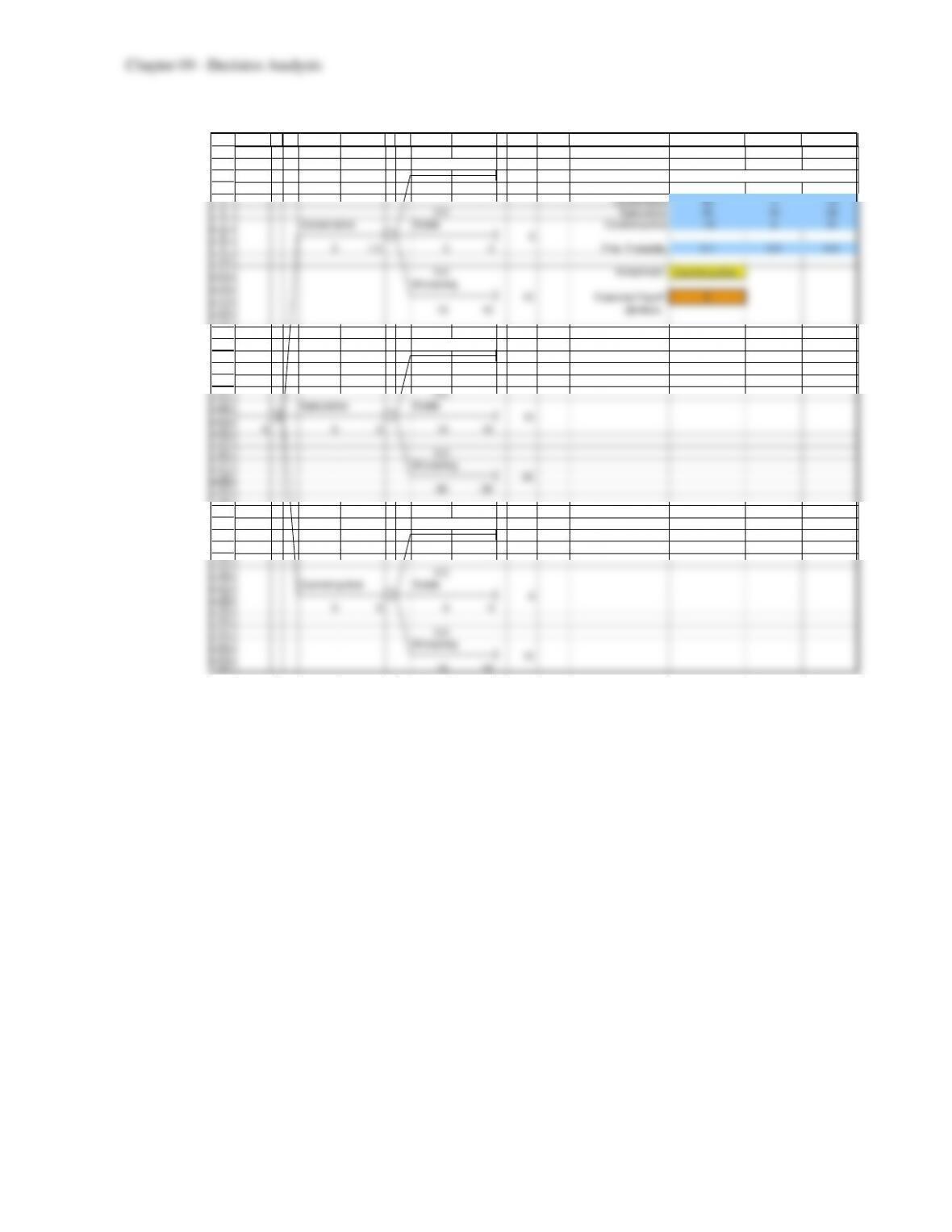
e)
1
2
3
4
5
6
7
8
9
10
11
12
13
14
15
16
17
18
19
20
21
22
23
24
25
26
27
28
29
30
31
32
33
34
35
36
37
38
39
40
41
42
43
44
A B C D E F G H I J K L M N O P
0.1
Improving Payoff T able ($million)
30 Alternative State of Nature (Economy)
30 30 (I nvest ment) I mproving St able W orsening
Conservative 30 5 -10
0.5 Speculative 40 10 -30
Conservative Stable Countercyclical -10 0 15
5
0 1.5 5 5 Prior Probability 0.1 0.5 0.4
0.4 Investment Countercyclical
W orsening
-10 Expected Payoff 5
-10 -10 ($million)
0.1
Improving
40
40 40
0.5
Speculative Stable
310
5 0 -3 10 10
0.4
W orsening
-30
-30 -30
0.1
Improving
-10
-10 -10
0.5
Countercyclical Stable
0
0 5 0 0
0.4
W orsening
15
15 15
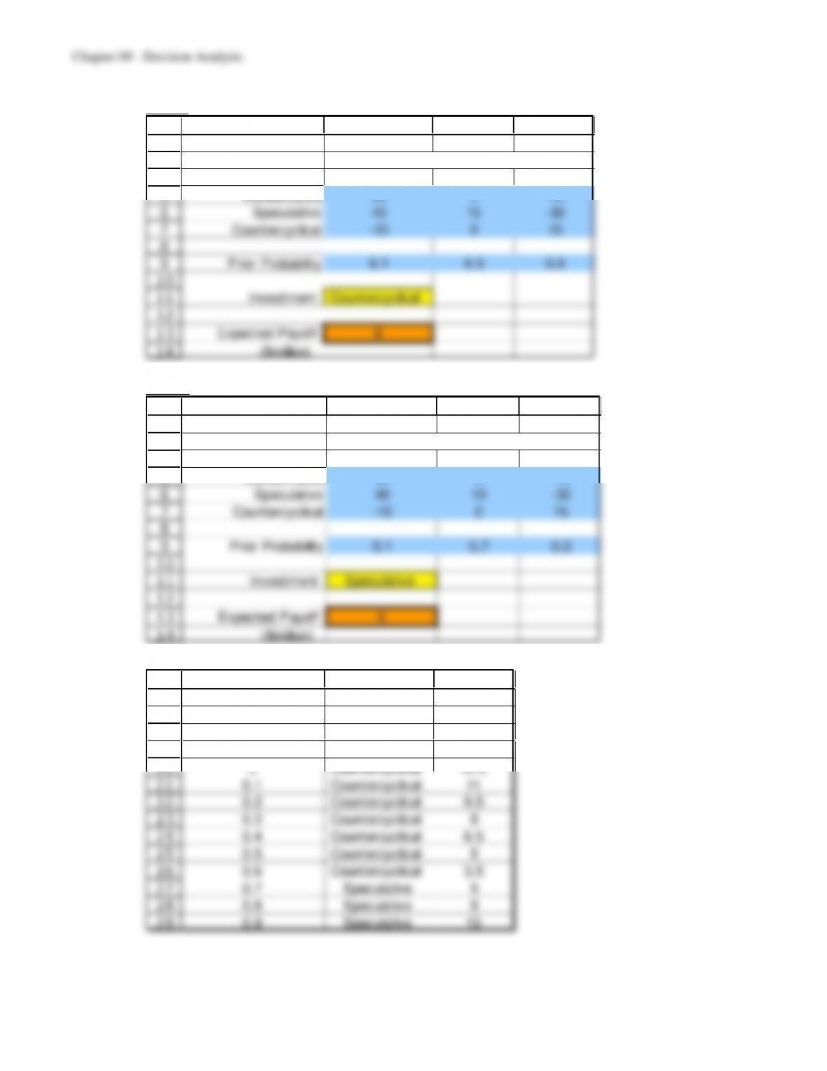
f) Part a)
2
3
4
5
6
7
8
9
10
11
12
13
14
M N O P
Payoff Table ($million)
Alternative State of Nature (Economy)
(Investment) Improving Stable Worsening
Conservative 30 5 -10
Speculative 40 10 -30
Countercyclical -10 0 15
Prior Probability 0.1 0.3 0.6
Investment Countercyclical
Expected Payoff 8
($million)
Part b)
2
3
4
5
6
7
8
9
10
11
12
13
14
M N O P
Payoff Table ($million)
Alternative State of Nature (Economy)
(Investment) Improving Stable Worsening
Conservative 30 5 -10
Speculative 40 10 –30
Countercyclical -10 0 15
Prior Probability 0.1 0.7 0.2
Investment Speculative
Expected Payoff 5
($million)
g)
16
17
18
19
20
21
22
23
24
25
26
27
M N O
Expected
Probability of Optimal Payoff
Stable Economy Investment ($million)
Speculative 5
0 Countercyclical 12.5
0.1 Countercyclical 11
0.2 Countercyclical 9.5
0.3 Countercyclical 8
0.4 Countercyclical 6.5
0.5 Countercyclical 5
0.6 Countercyclical 3.5
0.7 Speculative 5
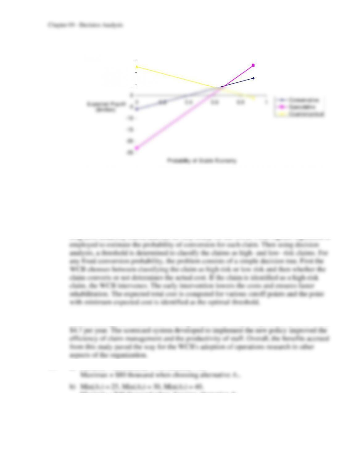
h)
-25
-20
-15
-10
-5
0
5
10
15
0 0.2 0.4 0.6 0.8 1
Probability of Stable Economy
Expected Payoff
($million)
Conservative
Speculative
Countercyclical
Counter-cyclical and conservative cross at approximately p=0.62.
Conservative and speculative cross at approximately p = 0.68.
9.6 This article describes the use of decision analysis at the Workers’ Compensation Board of
British Columbia (WCB), which is “responsible for the occupational health and safety,
rehabilitation, and compensation interests of British Columbia’s workers and employers”
[p. 15]. The focus of the study is on the short-term disability claims that can later turn into
long-term disability claims and can be very costly for the WCB. First, logistic regression is
The new policy offers accurate predictions of high-risk claims. As a result, future costs are
reduced and injured workers start working sooner. This study is expected to save the WCB
9.7 a) Max(A1) = 80, Max(A2) = 50, Max(A3) = 60.
Maximin = $40 thousand when choosing alternative A3.
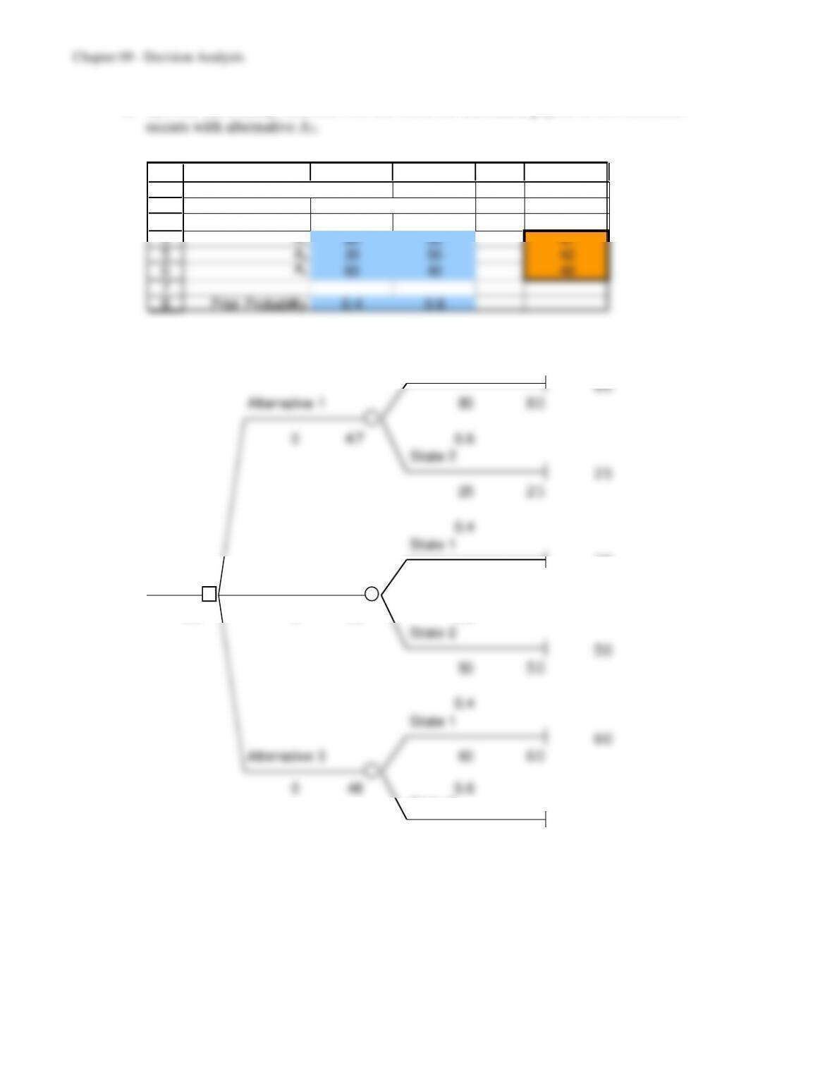
c) S2 is the most likely outcome. For this state, the maximum payoff of $50 thousand
d) Alternative A3 has the highest expected payoff of $48 thousand.
1
2
3
4
5
6
7
8
A B C D E
Payoff Table ($thousand) Expected
Payoff
Alternative
S1S2($thousand)
A180 25 47
A230 50 42
A360 40 48
Prior Probability 0.4 0.6
State of Nature
e)
0.4
State 1
80
Alternative 1 80 80
047 0.6
State 2
25
25 25
0.4
State 1
30
Alternative 2 30 30
3
048 0.6
State 2
40
40 40
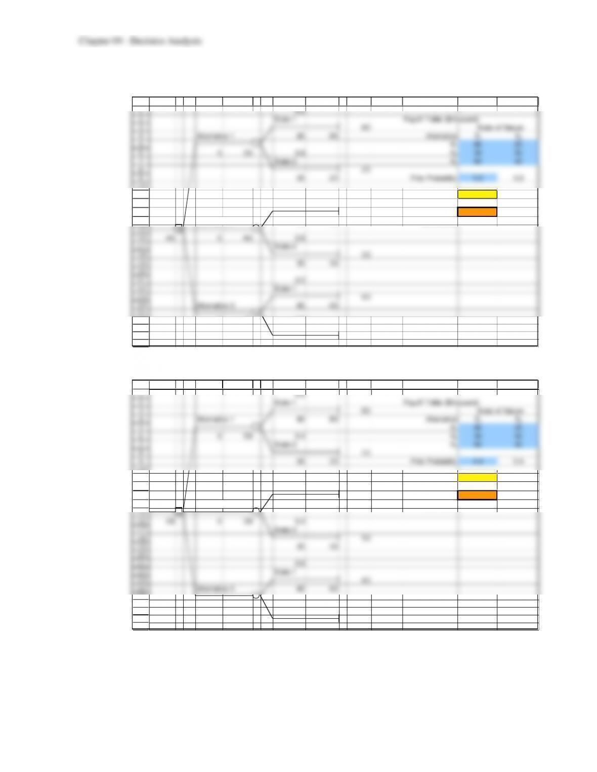
f) When the prior probability of S1 is 0.2, alternative A2 should be chosen, with an
expected payoff of $46 thousand.
1
2
3
4
5
6
7
8
9
10
11
12
13
14
15
16
17
18
19
20
21
22
23
24
25
26
27
28
29
A B C D E F G H I J K L M N O
0.2
State 1
80
Alternative 1 80 80 Alternative
S1S2
A180 25
036 0.8
A230 50
State 2
A360 40
25
25 25 Prior Probability 0.2 0.8
0.2 Best Alternative 2
State 1
30 Expected Payoff 46
Alternative 2 30 30 ($thousand)
2
46 046 0.8
State 2
50
50 50
0.2
State 1
60
Alternative 3 60 60
044 0.8
State 2
40
40 40
Payoff Table ($thousand)
State of Nature
When the prior probability of S1 is 0.6, alternative A1 should be chosen, with an
expected payoff of $58 thousand.
1
2
3
4
5
6
7
8
9
10
11
12
13
14
15
16
17
18
19
20
21
22
23
24
25
26
052 0.4
27
28
29
A B C D E F G H I J K L M N O
0.6
State 1
80
Alternative 1 80 80 Alternative
S1S2
A180 25
058 0.4
A230 50
State 2
A360 40
25
25 25 Prior Probability 0.6 0.4
0.6 Best Alternative 1
State 1
30 Expected Payoff 58
Alternative 2 30 30 ($thousand)
1
58 038 0.4
State 2
State 2
40
40 40
Payoff Table ($thousand)
State of Nature
g)
17
18
19
20
21
22
23
24
25
26
27
28
29
30
31
M N O
Prior Expected
Probability Best Payoff
of S
1Alternative ($thousand)
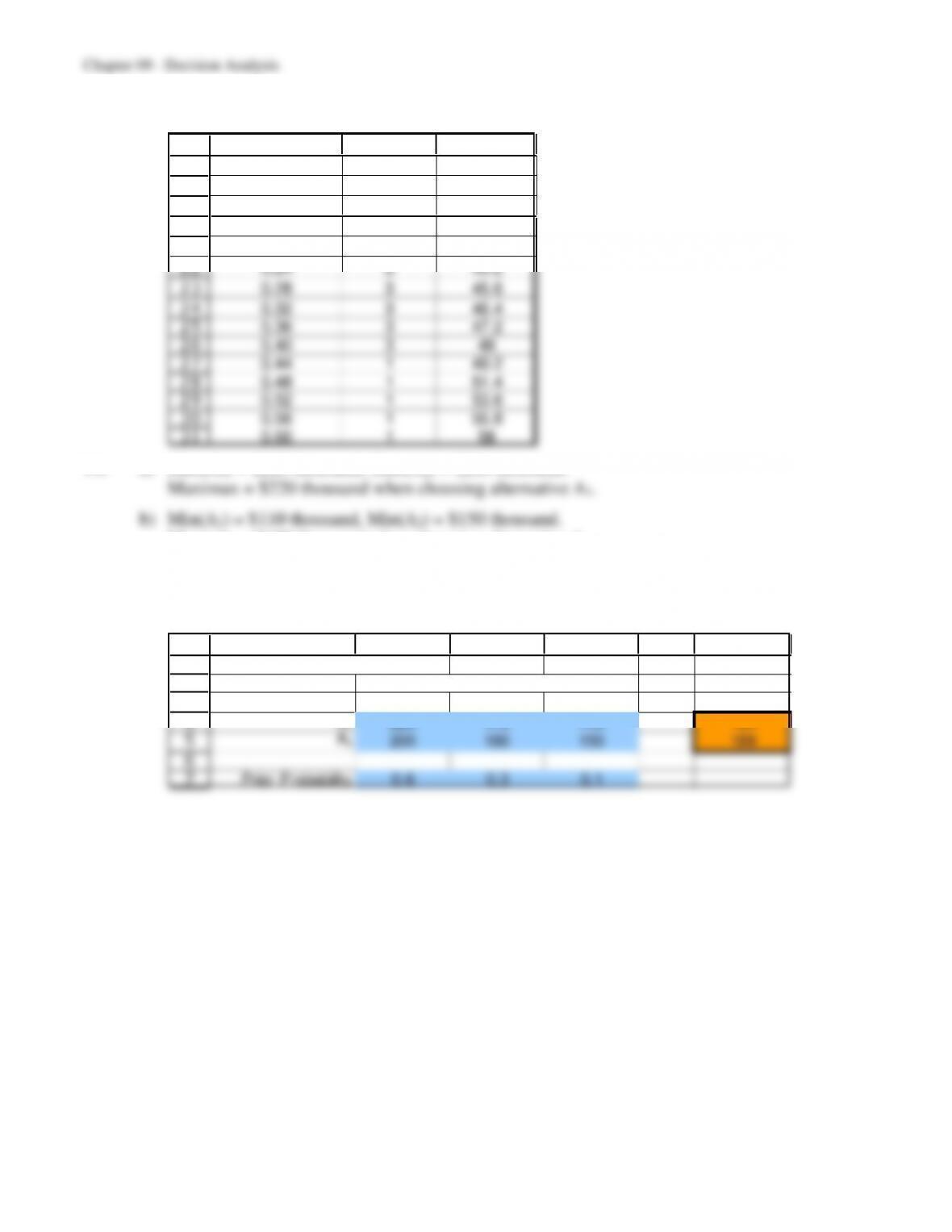
246
0.20 2 46
0.24 2 45.2
0.28 3 45.6
0.32 3 46.4
0.36 3 47.2
0.40 3 48
0.44 1 49.2
0.48 1 51.4
0.52 1 53.6
0.56 1 55.8
0.60 1 58
9.8 a) Max(A1) = $220 thousand, Max(A2) = $200 thousand.
Maximin = $150 thousand when choosing alternative A2.
c) S1 is the most likely outcome. For this state, the maximum payoff of $220 thousand
occurs with alternative A1.
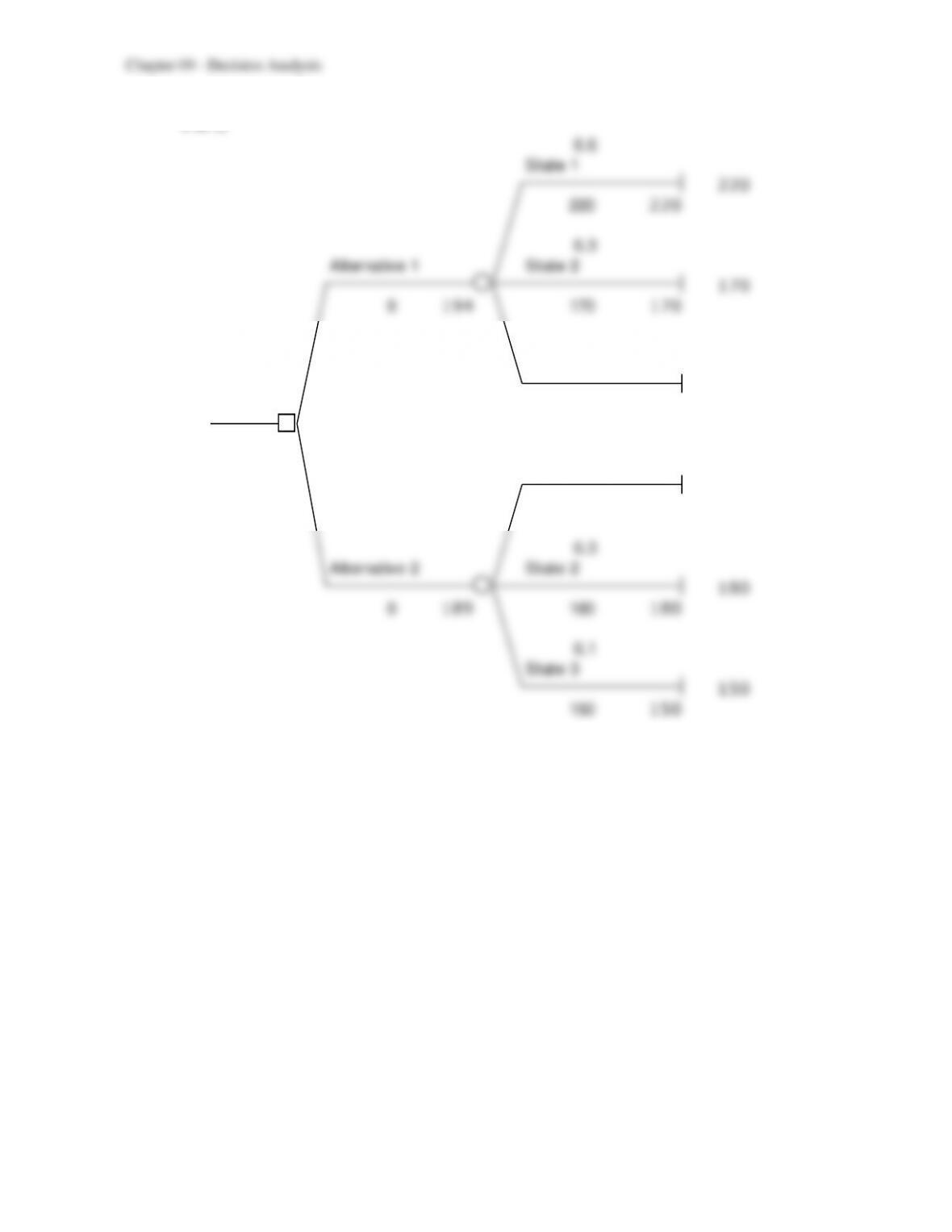
d) Alternative A1 has the highest expected payoff of $194 thousand.
1
2
3
4
5
6
7
A B C D E F
Payoff Table ($thousand) Expected
State of Nature Payoff
Alternative
S1S2S3($thousand)
A1220 170 110 194
A2200 180 150 189
Prior Probability 0.6 0.3 0.1
9-15
e & f)
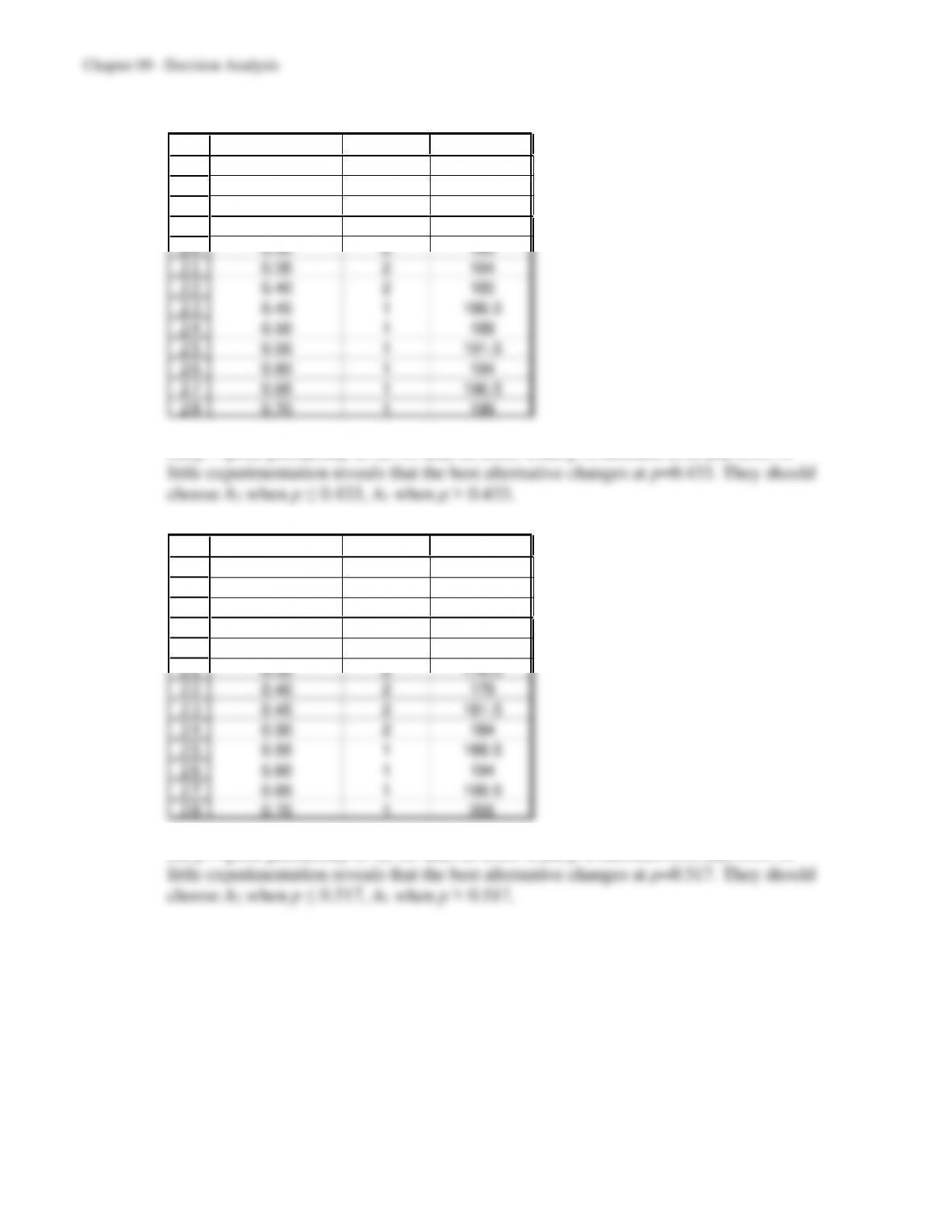
0.6
State 1
220
220 220
0.3
Alternative 1 State 2
170
0194 170 170
0.1
State 3
110
110 110
1
194 0.6
State 1
200
200 200
0.3
Alternative 2 State 2
180
0189 180 180
0.1
g)
16
17
18
19
20
21
22
23
24
25
26
27
28
M N O
Prior Expected
Probability Best Payoff
of S
1Alternative ($thousand)
1 194
0.30 2 183
0.35 2 184
0.40 2 185
0.45 1 186.5
0.50 1 189
0.55 1 191.5
0.60 1 194
0.65 1 196.5
0.70 1 199
Let p = prior probability of S1. A1 and A2 cross when p is between 0.40 and 0.45. A
h)
16
17
18
19
20
21
22
23
24
25
26
27
28
M N O
Prior Expected
Probability Best Payoff
of S
1Alternative ($thousand)
1 194
0.30 2 174
0.35 2 176.5
0.40 2 179
0.45 2 181.5
0.50 2 184
0.55 1 188.5
0.60 1 194
0.65 1 199.5
0.70 1 205
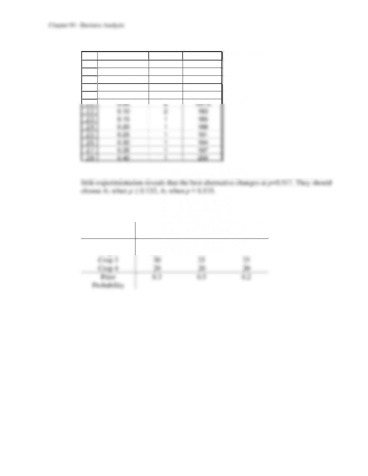
Let p = prior probability of S1. A1 and A2 cross when p is between 0.50 and 0.55. A
i)
16
17
18
19
20
21
22
23
24
25
26
27
28
M N O
Prior Expected
Probability Best Payoff
of S
2Alternative ($thousand)
1 194
0.00 2 180
0.05 2 181.5
0.10 2 183
0.15 1 185
0.20 1 188
0.25 1 191
0.30 1 194
0.35 1 197
0.40 1 200
Let p = prior probability of S2. A1 and A2 cross when p is between 0.10 and 0.15. A
j) Alternative A1 should be chosen.
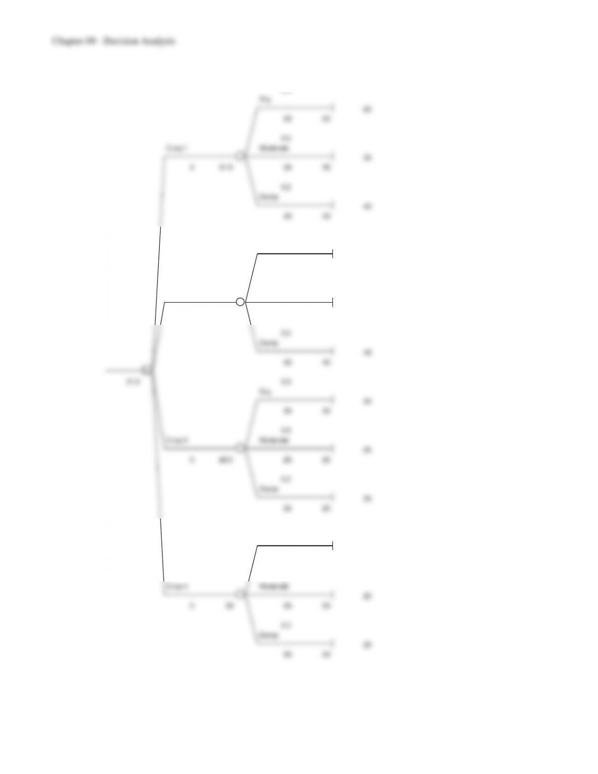
9.9 a)
State of Nature (Weather)
Alternative
Dry
Moderate
Damp
Crop 1
20
35
40
Crop 2
22.5
30
45
Crop 3
30
25
25
Crop 4
20
20
20
Prior
Probability
0.3
0.5
0.2
9-18
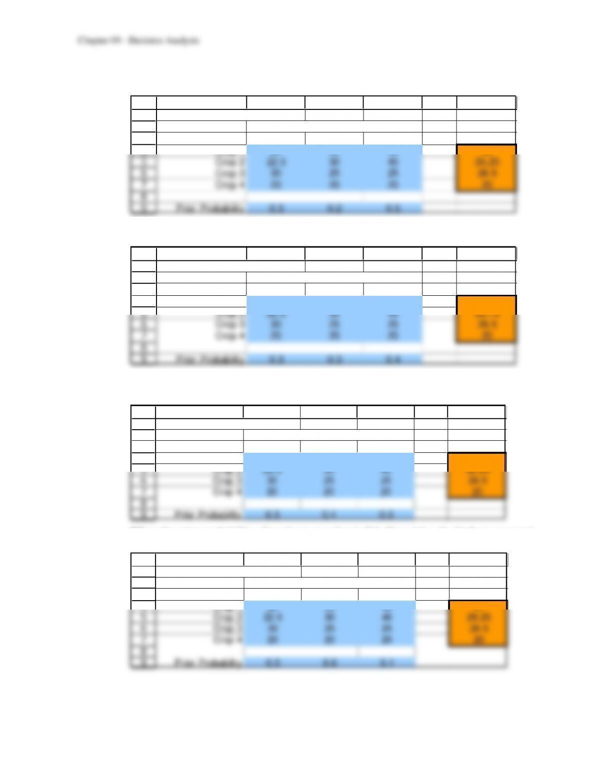
b) Crop 1 has the highest expected payoff of $31,500.
0.3
Dry
20
20 20
0.5
Crop 1 Moderate
35
0 31.5 35 35
0.2
Damp
40
Damp
45
45 45
1
31.5 0.3
Dry
30
30 30
0.5
Crop 3 Moderate
Damp
20
20 20
9-19
c) When the prior probability of moderate weather is 0.2, Crop 2 has the highest expected
payoff of $35,250.
1
2
3
4
5
6
7
8
9
A B C D E F
Payoff Table ($thousand) Expected
State of Nature (Weather) Payoff
Alternative Dry Moderate Damp ($thousand)
Crop 1 20 35 40 33
Crop 2 22.5 30 45 35.25
Crop 3 30 25 25 26.5
Crop 4 20 20 20 20
Prior Probability 0.3 0.2 0.5
When the prior probability of moderate weather is 0.3, Crop 2 has the highest expected
payoff of $33,750.
1
2
3
4
5
6
7
8
9
A B C D E F
Payoff Table ($thousand) Expected
State of Nature (Weather) Payoff
Alternative Dry Moderate Damp ($thousand)
Crop 1 20 35 40 32.5
Crop 2 22.5 30 45 33.75
Crop 3 30 25 25 26.5
Crop 4 20 20 20 20
Prior Probability 0.3 0.3 0.4
When the prior probability of moderate weather is 0.4, Crop 2 has the highest expected
payoff of $32,250.
1
2
3
4
5
6
7
8
9
A B C D E F
Payoff Table ($thousand) Expected
State of Nature (Weather) Payoff
Alternative Dry Moderate Damp ($thousand)
Crop 1 20 35 40 32
Crop 2 22.5 30 45 32.25
Crop 3 30 25 25 26.5
Crop 4 20 20 20 20
Prior Probability 0.3 0.4 0.3
When the prior probability of moderate weather is 0.6, Crop 1 has the highest expected
payoff of $31,000.
1
2
3
4
5
6
7
8
9
A B C D E F
Payoff Table ($thousand) Expected
State of Nature (Weather) Payoff
Alternative Dry Moderate Damp ($thousand)
Crop 1 20 35 40 31
Crop 2 22.5 30 45 29.25
Crop 3 30 25 25 26.5
Crop 4 20 20 20 20
Prior Probability 0.3 0.6 0.1