8-21
b & c) The profit graph for product 1 is shown below.
Product i on of product 1
Profit
($mi ll ions)
5
1 2 3 4 5
4
3
1
-1
2
The profit graph for product 2 is shown below.
Product i on of product 2
Profi t
($mi ll ions)
10
1 2 3 4 5
8
6
4
2
-2
-4
8-22
d)
1
2
3
4
5
6
7
8
9
10
11
12
13
14
15
16
17
18
A B C D E F
Unit Profit ($millions) Campaign 1 Campaign 2
0 to 2 3 5
2 to 4 -1 1
4 to 5 -4 -2
Total Resource
Used Available
Resource 1 4 1 12 <= 20
Resource 2 1 4 18 <= 20
Campaign 1 Campaign 2 Campaign 1 Campaign 2
0 to 2 2 2 <= 2 2
2 to 4 0 2 <= 2 2
4 to 5 0 0 <= 1 1
Total 2 4
Total Profit
($millions)
18
Maximum
Resource Used per Unit
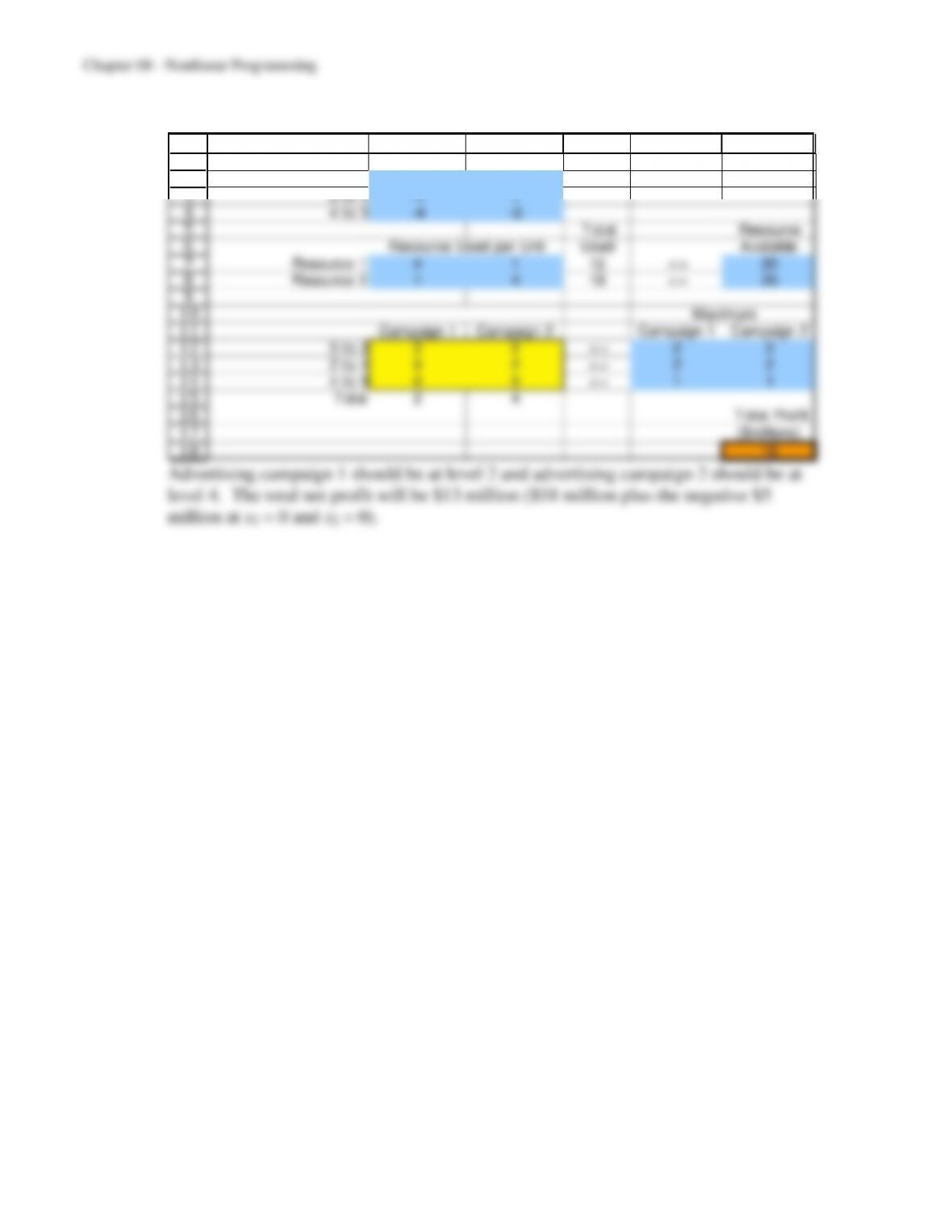
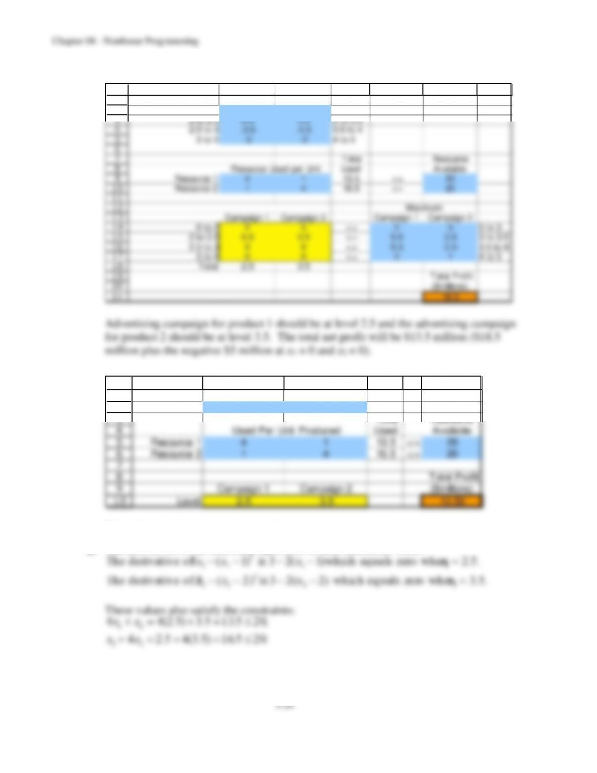
Advertising campaign 1 should be at level 2 and advertising campaign 2 should be at
level 4. The total net profit will be $13 million ($18 million plus the negative $5
million at x1 = 0 and x2 = 0).
8-23
e) The revised approximated profit graph for product 1 is shown below.
Product i on of product 1
Profit
($mi ll ions)
5
1 2 3 4 5
4
3
1
-1
2
The profit graph for product 2 is shown below.
Product ion of product 2
Profit
($mil lions)
10
1 2 3 4 5
8
6
4
2
-2
-4
The linear programming model is then as follows:
8.15 a)
1
2
3
4
5
6
7
8
9
A B C D E F
0 Starting
<= Point x* Profit*
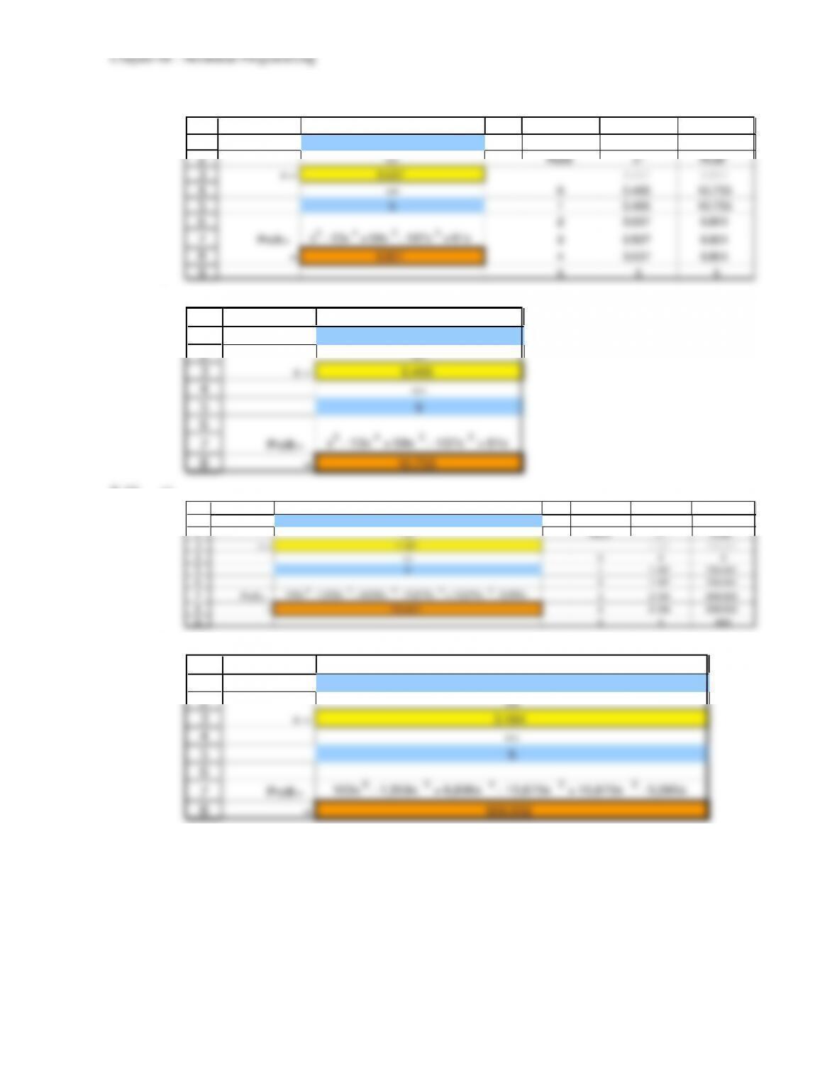
x = 3.537 3.537 6.801
<= 0 0.405 10.735
5 1 0.405 10.735
2 3.537 6.801
Profit =
x5 – 13x 4 + 59x 3 – 107x 2 + 61x 3 3.537 6.801
= 6.801 4 3.537 6.801
5 5 5
b)
1
2
3
4
5
6
7
8
A B
0
<=
x = 0.405
<=
5
Profit =
x5 – 13x 4 + 59x 3 – 107x 2 + 61x
= 10.735
8.16 a)
1
2
3
4
5
6
7
8
9
A B C D E F
0 Starting
<= Point x* Profit*
x = 1.187 1.187 753.451
<= 0 0 0
5 1 1.187 753.451
2 1.187 753.451
Profit =
100x 6 – 1,359x 5 + 6,836x 4 – 15,670x 3 + 15,870x 2 – 5,095x 3 3.184 906.902
= 753.451 4 3.184 906.902
5 5 650
b)
1
2
3
4
5
6
7
8
A B
0
<=
x = 3.184
<=
5
Profit =
100x 6 – 1,359x 5 + 6,836x 4 – 15,670x 3 + 15,870x 2 – 5,095x
= 906.902
8.17
1
2
3
4
5
6
7
8
9
10
11
12
13
14
15
16
17
18
19
20
A B C D E F G H I J K L M N O P
City Democrat Republican Total District
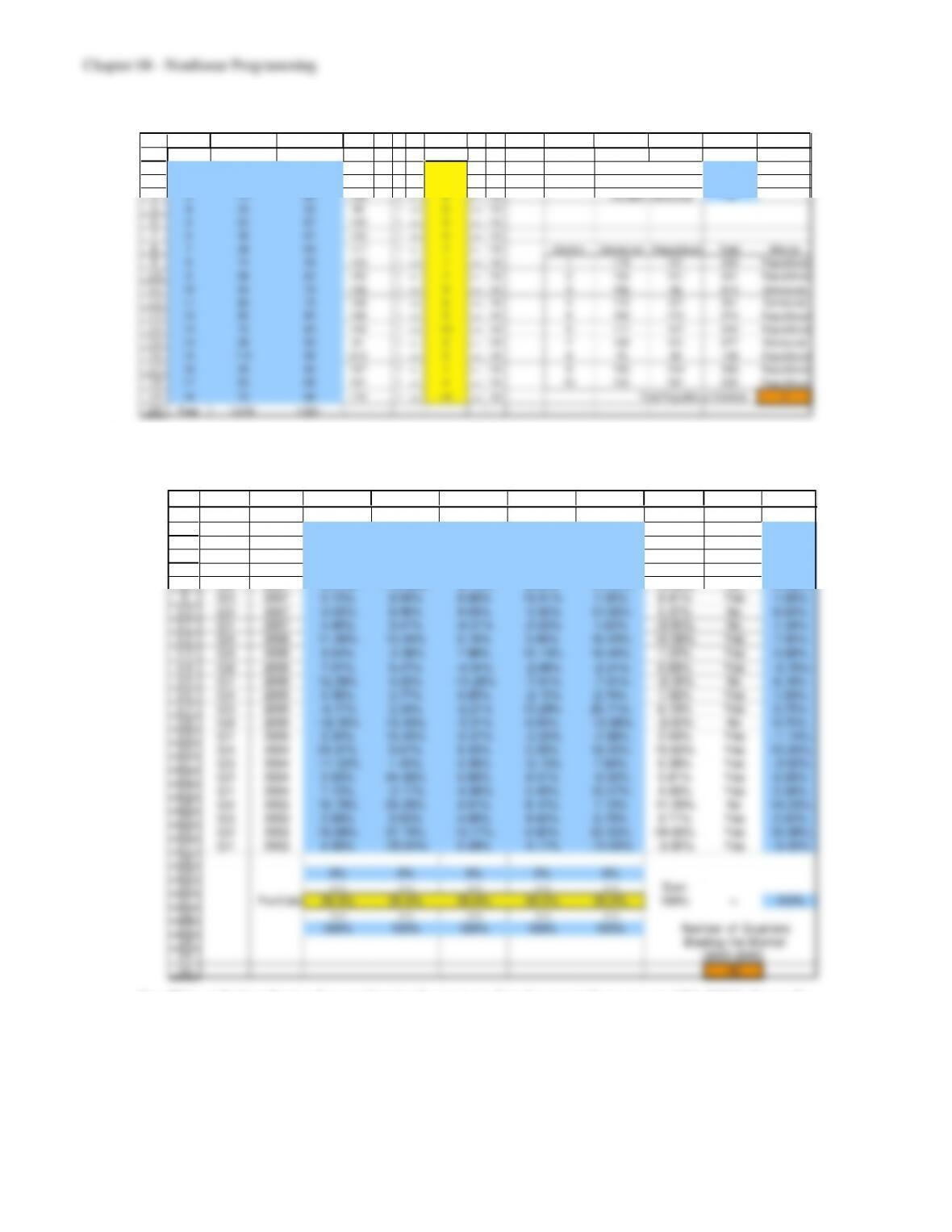
1 152 62 214 1 <= 3<= 10 Min District Population 150
281 59 140 1 <= 4<= 10 Max District Population 350
375 83 158 1 <= 8<= 10 Number of Districts 10
434 52 86 1<= 6<= 10
562 87 149 1 <= 5<= 10
638 87 125 1 <= 5<= 10
748 69 117 1 <= 7<= 10 District Democrat Republican Total Winner
874 49 123 1 <= 1<= 10 1 119 131 250 Republican
998 62 160 1 <= 7<= 10 2 140 151 291 Republican
10 66 72 138 1 <= 9<= 10 3 152 62 214 Democrat
11 83 75 158 1 <= 6<= 10 4 174 127 301 Democrat
12 86 82 168 1 <= 9<= 10 5 100 174 274 Republican
13 72 83 155 1 <= 10 <= 10 6 117 127 244 Republican
14 28 53 81 1<= 2<= 10 7 146 131 277 Democrat
15 112 98 210 1 <= 2<= 10 875 83 158 Republican
16 45 82 127 1 <= 1<= 10 9 152 154 306 Republican
17 93 68 161 1 <= 4<= 10 10 144 181 325 Republican
18 72 98 170 1 <= 10 <= 10 Total Republican Districts 7
Total 1,319 1,321
8.18 a) Interestingly, the starting point solution (20% in each stock) proves to be a very good
solution (beating the NYSE in 10 of the 12 quarters) and Evolutionary Solver did not
improve on this solution.
3
4
5
6
7
8
9
10
11
12
13
14
15
16
17
18
19
20
21
22
23
24
25
26
27
28
29
30
31
32
33
34
35
36
B C D E F G H I J K
Quarter Year DIS BA GE PG MCD Return Market? (NYSE)
Q4 2008 -24.97% -25.05% –35.26% –10.73% 1.68% –18.86% Yes -23.57%
Q3 2008 -1.63% -12.19% –3.17% 15.33% 10.42% 1.75% Yes -13.02%
Q2 2008 -0.58% –11.22% -27.07% –12.72% 1.47% –10.02% No –1.56%
Q1 2008 -2.77% -14.55% 0.74% -4.08% –4.69% -5.07% Yes –9.68%
Q4 2007 -5.13% -16.40% –9.70% 4.90% 11.01% -3.06% No -2.98%
Q3 2007 0.72% 9.56% 8.88% 15.61% 7.30% 8.41% Yes 1.68%
Q2 2007 -0.83% 8.56% 9.05% -2.60% 12.66% 5.37% No 6.60%
Q1 2007 0.48% 0.47% -4.21% –2.63% 1.62% -0.85% No 1.34%
Q4 2006 11.86% 13.06% 6.18% 5.69% 16.09% 10.58% Yes 7.90%
Q3 2006 3.04% -3.36% 7.88% 12.10% 16.44% 7.22% Yes 3.68%
Q2 2006 7.57% 5.47% -4.54% –2.98% –2.21% 0.66% Yes –0.78%
Q1 2006 12.39% 4.05% -13.25% –7.51% –7.41% -2.35% No 6.18%
Q4 2005 0.38% 3.77% 4.85% -2.15% 2.74% 1.92% Yes 1.59%
Q3 2005 -4.17% 3.34% -2.21% 13.29% 20.71% 6.19% Yes 5.75%
Q2 2005 -12.35% 13.36% -3.31% 0.04% -10.88% -2.63% No 0.70%
Q1 2005 3.34% 13.45% -0.57% –3.33% -2.90% 2.00% Yes –1.14%
Q4 2004 24.37% 0.67% 9.32% 2.26% 16.50% 10.62% Yes 10.35%
Q3 2004 -11.52% 1.45% 4.26% -0.13% 7.84% 0.38% Yes -0.50%
Q2 2004 2.00% 24.99% 6.80% 4.31% –9.02% 5.81% Yes 0.06%
Q1 2004 7.12% -2.17% -0.89% 5.49% 15.07% 4.93% Yes 2.09%
Q4 2003 16.79% 23.28% 4.61% 8.12% 7.13% 11.99% No 14.53%
Q3 2003 2.08% 0.55% 4.60% 4.64% 6.70% 3.71% Yes 2.52%
Q2 2003 16.09% 37.76% 13.17% 0.60% 52.55% 24.03% Yes 16.38%
Q1 2003 4.36% -23.61% 5.59% 4.11% –10.05% -3.92% Yes –5.40%
0% 0% 0% 0% 0%
<= <= <= <= <= Sum
Portfolio 20.0% 20.0% 20.0% 20.0% 20.0% 100% = 100%
<= <= <= <= <=
100% 100% 100% 100% 100% Number of Q uarters
Beating the Market
(2003-2005)
10
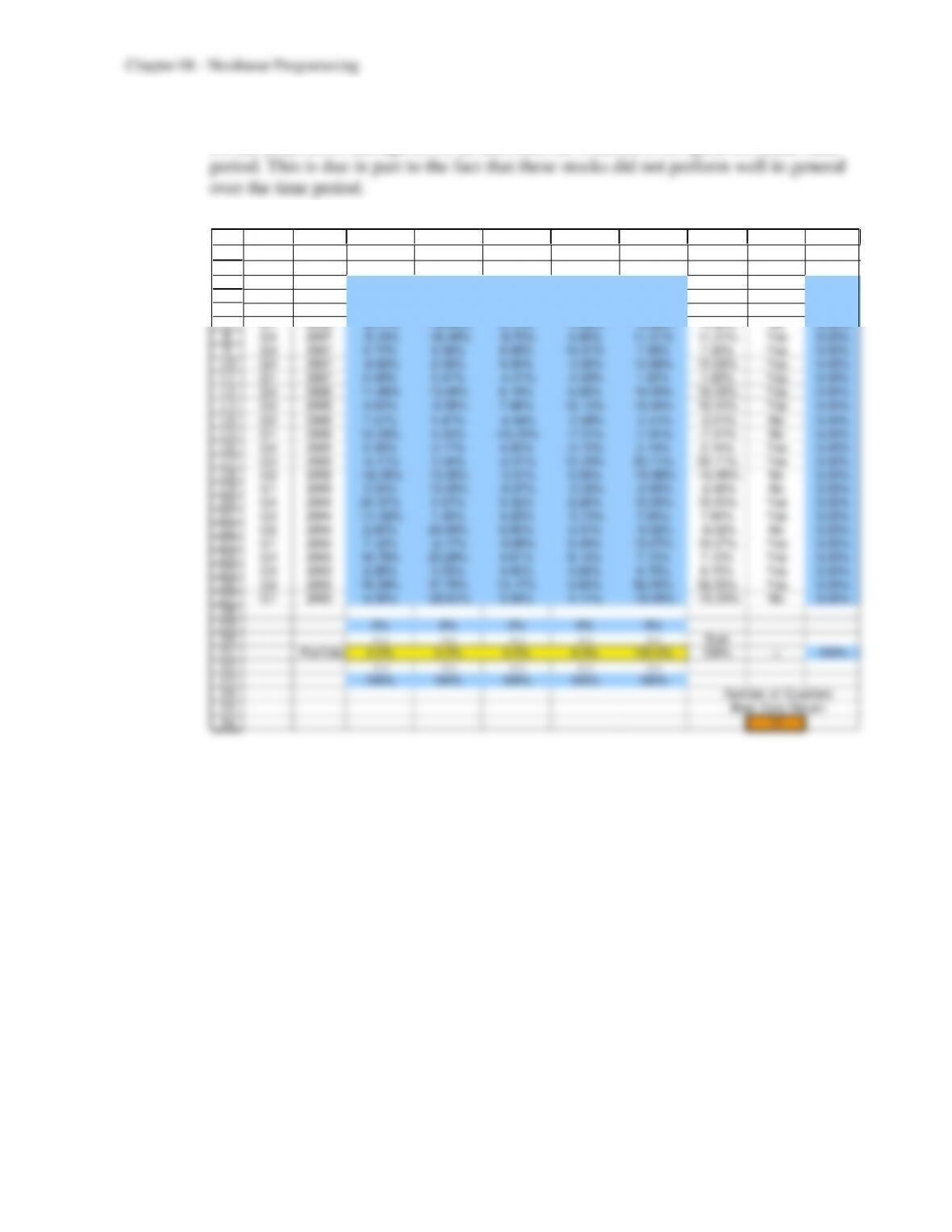
b) This solution beats the market in 7 quarters for the next three years (Q1 2006 through
8-27
c) The optimized solution for years 2003 through 2005 is not necessarily a good solution
for the years 2006 through 2008. In this case, the solution is not great for either time
8.19 a) Answers may vary since Evolutionary Solver is based on randomness.
2
3
4
5
6
7
8
9
10
11
12
13
14
15
16
17
18
19
20
21
22
23
24
25
26
27
28
29
30
31
32
33
34
35
36
B C D E F G H I J K
Beat Z ero
Quarter Year DIS BA GE PG MCD Return Zero? Return
Q4 2008 -24.97% -25.05% -35.26% -10.73% 1.68% 1.68% Yes 0.00%
Q3 2008 –1.63% -12.19% –3.17% 15.33% 10.42% 10.42% Yes 0.00%
Q2 2008 –0.58% –11.22% -27.07% -12.72% 1.47% 1.47% Yes 0.00%
Q1 2008 –2.77% -14.55% 0.74% -4.08% –4.69% -4.69% No 0.00%
Q4 2007 –5.13% -16.40% –9.70% 4.90% 11.01% 11.01% Yes 0.00%
Q3 2007 0.72% 9.56% 8.88% 15.61% 7.30% 7.30% Yes 0.00%
Q2 2007 –0.83% 8.56% 9.05% -2.60% 12.66% 12.66% Yes 0.00%
Q1 2007 0.48% 0.47% -4.21% –2.63% 1.62% 1.62% Yes 0.00%
Q4 2006 11.86% 13.06% 6.18% 5.69% 16.09% 16.09% Yes 0.00%
Q3 2006 3.04% -3.36% 7.88% 12.10% 16.44% 16.44% Yes 0.00%
Q2 2006 7.57% 5.47% -4.54% –2.98% -2.21% -2.21% No 0.00%
Q1 2006 12.39% 4.05% –13.25% –7.51% -7.41% -7.41% No 0.00%
Q4 2005 0.38% 3.77% 4.85% –2.15% 2.74% 2.74% Yes 0.00%
Q3 2005 –4.17% 3.34% –2.21% 13.29% 20.71% 20.71% Yes 0.00%
Q2 2005 -12.35% 13.36% -3.31% 0.04% -10.88% -10.88% No 0.00%
Q1 2005 3.34% 13.45% –0.57% -3.33% –2.90% -2.90% No 0.00%
Q4 2004 24.37% 0.67% 9.32% 2.26% 16.50% 16.50% Yes 0.00%
Q3 2004 -11.52% 1.45% 4.26% -0.13% 7.84% 7.84% Yes 0.00%
Q2 2004 2.00% 24.99% 6.80% 4.31% -9.02% -9.02% No 0.00%
Q1 2004 7.12% -2.17% -0.89% 5.49% 15.07% 15.07% Yes 0.00%
Q4 2003 16.79% 23.28% 4.61% 8.12% 7.13% 7.13% Yes 0.00%
Q3 2003 2.08% 0.55% 4.60% 4.64% 6.70% 6.70% Yes 0.00%
Q2 2003 16.09% 37.76% 13.17% 0.60% 52.55% 52.55% Yes 0.00%
Q1 2003 4.36% –23.61% 5.59% 4.11% -10.05% -10.05% No 0.00%
0% 0% 0% 0% 0%
<= <= <= <= <= Sum
Portfolio 0.0% 0.0% 0.0% 0.0% 100.0% 100% = 100%
<= <= <= <= <=
100% 100% 100% 100% 100%
Number of Q uarters
Beat Zero Return
17
Chapter 08 – Nonlinear Programming
8-28
b) Answers may vary since Evolutionary Solver is based on randomness.
2
3
4
5
6
7
8
9
10
11
12
13
14
15
16
17
18
19
20
21
22
23
24
25
26
27
28
29
30
31
32
33
34
35
36
B C D E F G H I J K
Beat T en
Quarter Year DIS BA GE PG MCD Return Ten? Return
Q4 2008 -24.97% -25.05% -35.26% -10.73% 1.68% 1.68% No 10.00%
Q3 2008 –1.63% -12.19% –3.17% 15.33% 10.42% 10.42% Yes 10.00%
Q2 2008 –0.58% –11.22% -27.07% -12.72% 1.47% 1.47% No 10.00%
Q1 2008 –2.77% -14.55% 0.74% -4.08% –4.69% -4.69% No 10.00%
Q4 2007 –5.13% -16.40% –9.70% 4.90% 11.01% 11.01% Yes 10.00%
Q3 2007 0.72% 9.56% 8.88% 15.61% 7.30% 7.30% No 10.00%
Q2 2007 -0.83% 8.56% 9.05% -2.60% 12.66% 12.66% Yes 10.00%
Q1 2007 0.48% 0.47% -4.21% -2.63% 1.62% 1.62% No 10.00%
Q4 2006 11.86% 13.06% 6.18% 5.69% 16.09% 16.09% Yes 10.00%
Q3 2006 3.04% -3.36% 7.88% 12.10% 16.44% 16.44% Yes 10.00%
Q2 2006 7.57% 5.47% -4.54% –2.98% -2.21% -2.21% No 10.00%
Q1 2006 12.39% 4.05% –13.25% –7.51% -7.41% -7.41% No 10.00%
Q4 2005 0.38% 3.77% 4.85% –2.15% 2.74% 2.74% No 10.00%
Q3 2005 –4.17% 3.34% –2.21% 13.29% 20.71% 20.71% Yes 10.00%
Q2 2005 -12.35% 13.36% -3.31% 0.04% -10.88% -10.88% No 10.00%
Q1 2005 3.34% 13.45% –0.57% -3.33% –2.90% -2.90% No 10.00%
Q4 2004 24.37% 0.67% 9.32% 2.26% 16.50% 16.50% Yes 10.00%
Q3 2004 -11.52% 1.45% 4.26% -0.13% 7.84% 7.84% No 10.00%
Q2 2004 2.00% 24.99% 6.80% 4.31% -9.02% -9.02% No 10.00%
Q1 2004 7.12% -2.17% -0.89% 5.49% 15.07% 15.07% Yes 10.00%
Q4 2003 16.79% 23.28% 4.61% 8.12% 7.13% 7.13% No 10.00%
Q3 2003 2.08% 0.55% 4.60% 4.64% 6.70% 6.70% No 10.00%
Q2 2003 16.09% 37.76% 13.17% 0.60% 52.55% 52.55% Yes 10.00%
Q1 2003 4.36% –23.61% 5.59% 4.11% -10.05% -10.05% No 10.00%
0% 0% 0% 0% 0%
<= <= <= <= <= Sum
Portfolio 0.0% 0.0% 0.0% 0.0% 100.0% 100% = 100%
<= <= <= <= <=
100% 100% 100% 100% 100%
Number of Q uarters
Beat 10% Return
9
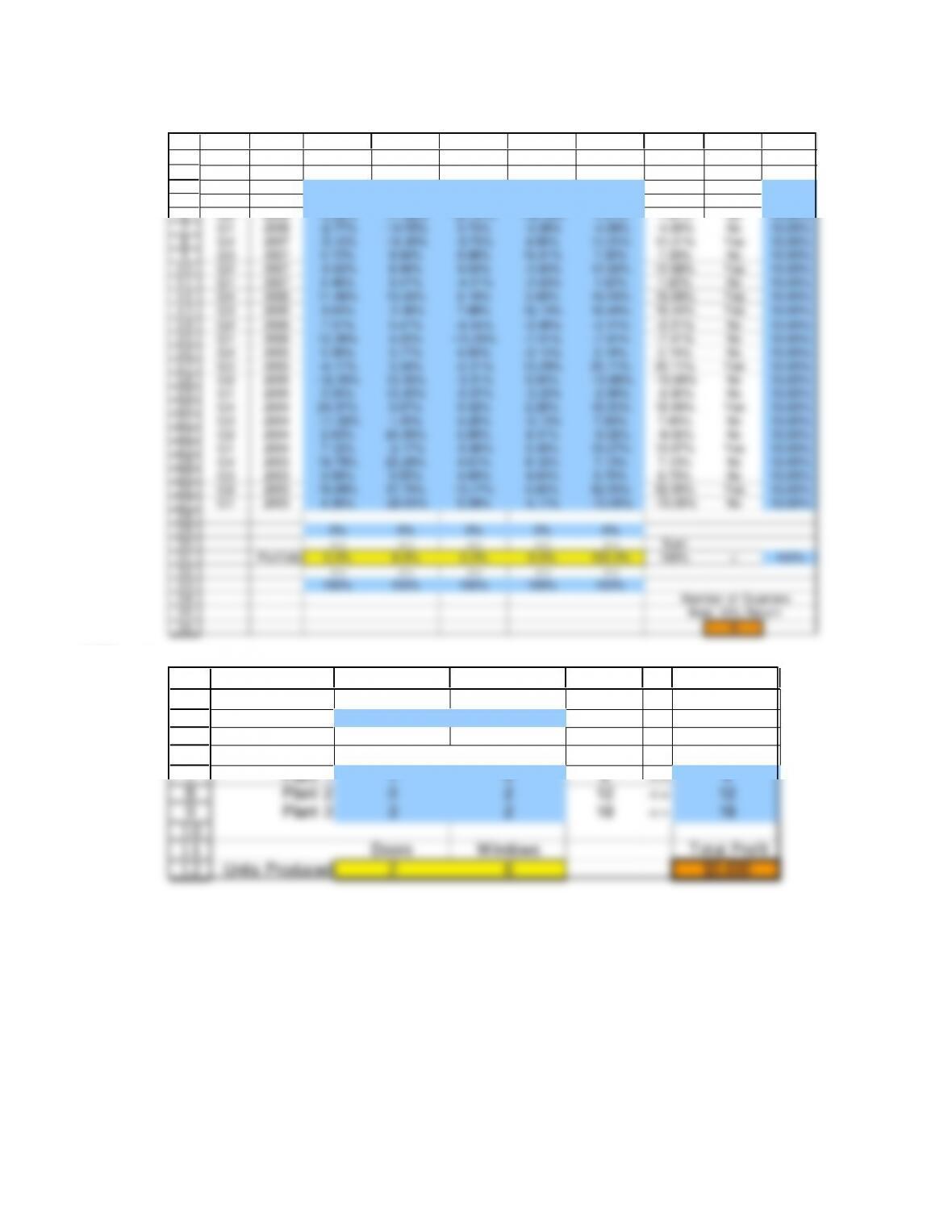
8.20 a)
3
4
5
6
7
8
9
10
11
12
B C D E F G
Doors Windows
Unit Profit $300 $500
Hours Hours
Used Available
Plant 1 1 0 2 <= 4
Plant 2 0 2 12 <= 12
Plant 3 3 2 18 <= 18
Doors W indows Total Profit
Units Produced 2 6 $3,600
Hours Used Per Unit Produced
8-29
b)
3
4
5
6
7
8
9
10
11
12
13
14
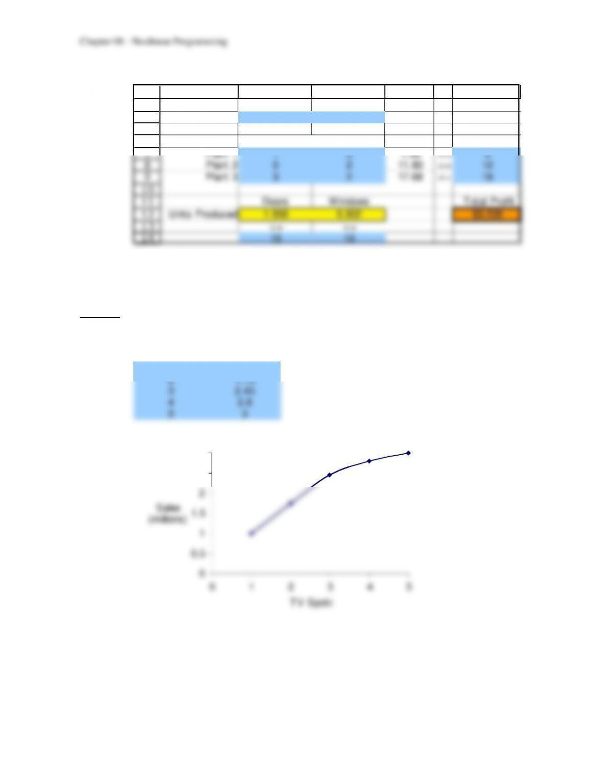
B C D E F G
Doors Windows
Unit Profit $300 $500
Hours Hours
Used Available
Plant 1 1 0 1.96 <= 4
Plant 2 0 2 11.80 <= 12
Plant 3 3 2 17.68 <= 18
Doors Windows Total Profit
Units Produced 1.959 5.902 $3,538
<= <=
Hours Used Per Unit Produced
c) The standard Solver gives a better solution and finds it much more quickly. The
standard Solver is much better suited to linear programs than is the Evolutionary
Solver.
Cases
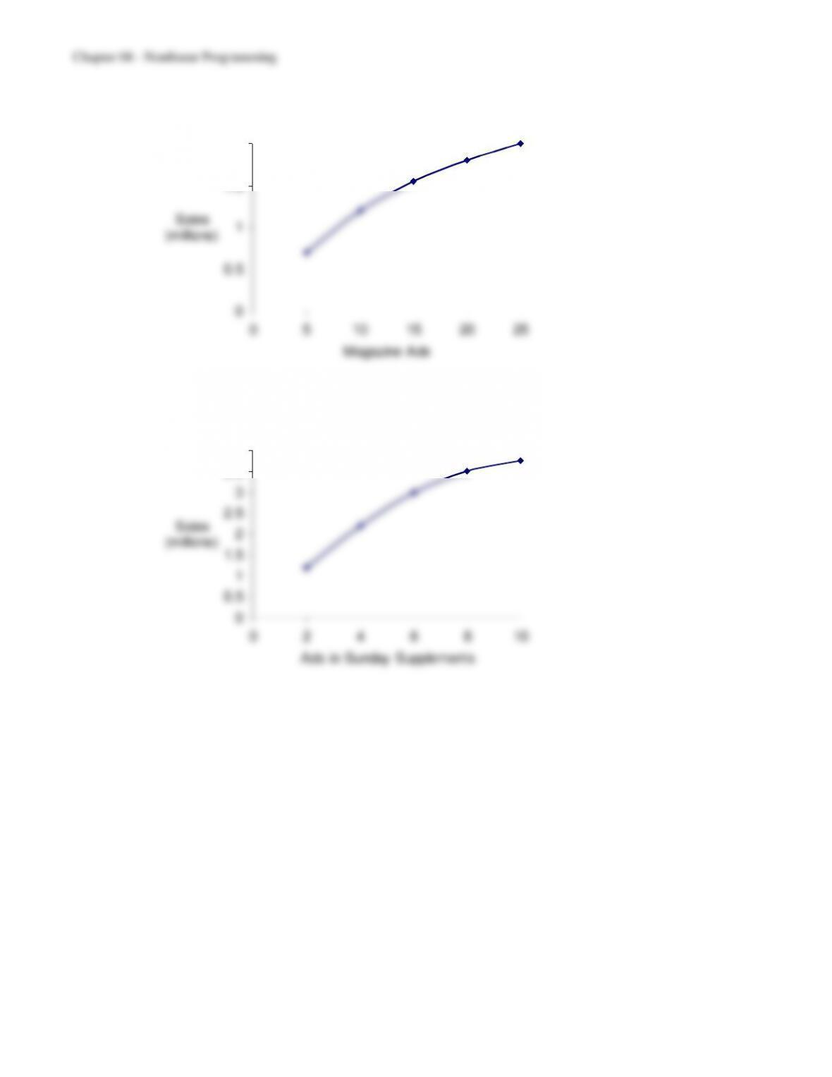
8-1 a) TV Spots
Sales
TV Spots (millions)
1 1
2 1.75
3 2.45
4 2.8
5 3
0
0.5
1
1.5
2
2.5
3
0 1 2 3 4 5
TV Spots
Sales
(millions)
8-30
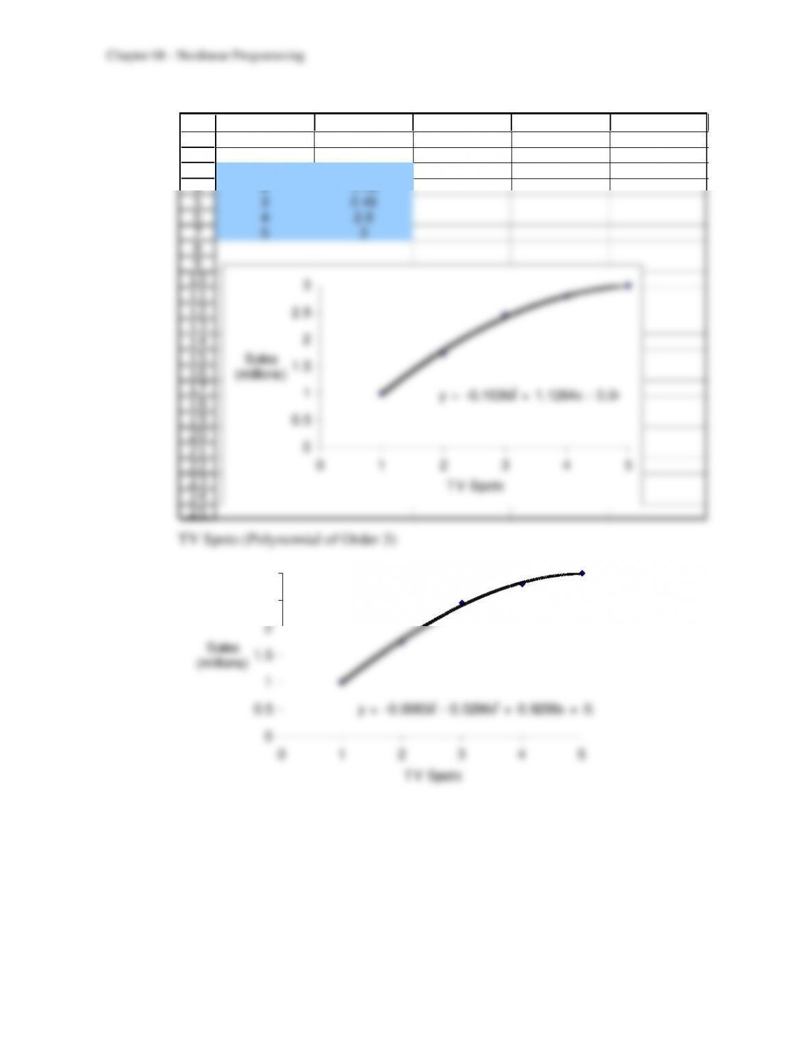
Magazine Ads
0
0.5
1
1.5
2
0 5 10 15 20 25
Magazine Ads
Sales
(millions)
Ads in Sunday Supplements
0
0.5
1
1.5
2
2.5
3
3.5
4
0 2 4 6 8 10
Ads in Sunday Supplements
Sales
(millions)
8-31
b) TV Spots (Polynomial of Order 2)
1
2
3
4
5
6
7
8
9
10
11
12
13
14
15
16
17
18
19
20
21
22
23
24
25
A B C D E
Sales
TV Spots (millions)
1 1
2 1.75
3 2.45
4 2.8
5 3
y = -0.1036x
2 + 1.1264x – 0.04
0
0.5
1
1.5
2
2.5
3
0 1 2 3 4 5
TV Spots
Sales
(millions)
TV Spots (Polynomial of Order 3)
y = -0.0083x
3 – 0.0286x
2 + 0.9298x + 0.1
0
0.5
1
1.5
2
2.5
3
0 1 2 3 4 5
TV Spots
Sales
(millions)
8-32
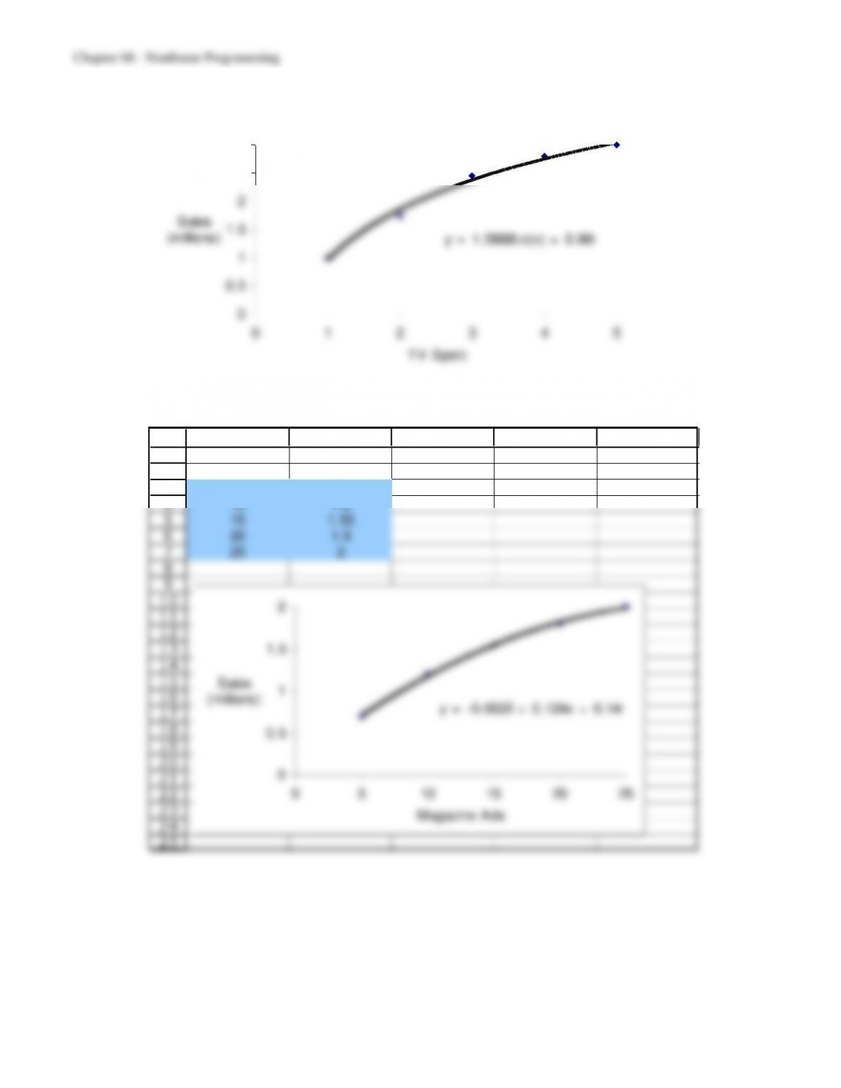
TV Spots (Logarithmic Form)
y = 1.2888Ln(x) + 0.966
0
0.5
1
1.5
2
2.5
3
0 1 2 3 4 5
TV Spots
Sales
(millions)
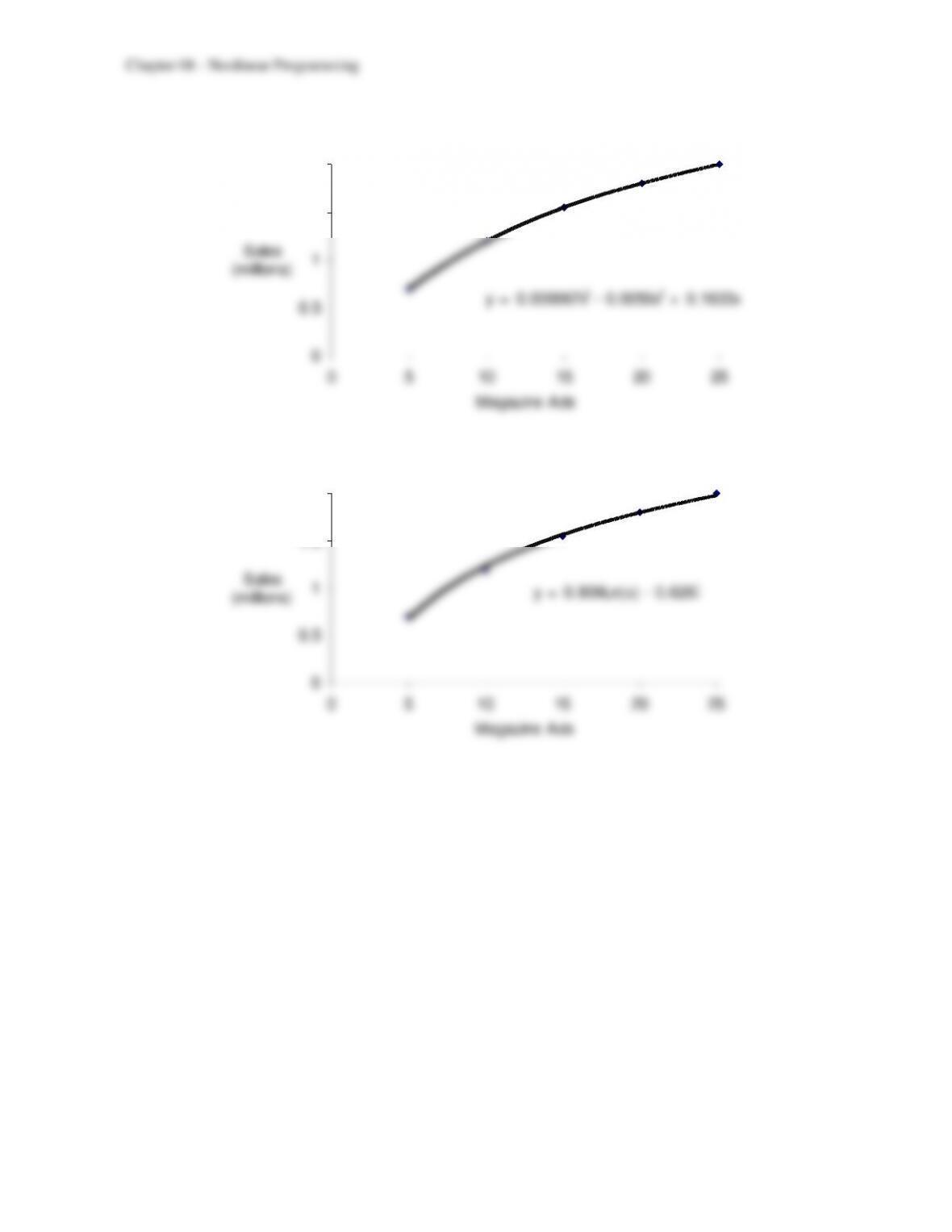
Magazine Ads (Polynomial of Order 2)
1
2
3
4
5
6
7
8
9
10
11
12
13
14
15
16
17
18
19
20
21
22
23
24
25
A B C D E
Sales
Magazine Ads (millions)
5 0.7
10 1.2
15 1.55
20 1.8
25 2
y = -0.002x
2 + 0.124x + 0.140
0
0.5
1
1.5
2
0 5 10 15 20 25
Magazine Ads
Sales
(millions)
8-33
Magazine Ads (Polynomial of Order 3)
y = 0.000067x
3 – 0.0050x2 + 0.1633x
0
0.5
1
1.5
2
0 5 10 15 20 25
Magazine Ads
Sales
(millions)
Magazine Ads (Logarithmic Form)
y = 0.809Ln(x) – 0.6267
0
0.5
1
1.5
2
0 5 10 15 20 25
Magazine Ads
Sales
(millions)