8-1
Chapter 8 Nonlinear Programming
Review Questions
8.1-1 In both cases, decisions need to be made regarding the levels of a number of activities,
where these activity levels can have any value that satisfies a number of constraints. The
decisions regarding activity levels are to be based on an overall measure of performance.
8.1-3 (1) Nonlinear programming is used to model nonproportional relationships between
activity levels and the overall measure of performance, whereas linear programming
8.1-4 The contribution of each activity to the value of the objective function is proportional to
the level of the activity in a linear program. When an activity has a nonproportional
8.1-6 This kind of graph might occur because overtime needs to be used to increase the level of
the activity beyond the first kink.
8.1-7 It is common to assume a quadratic form or a logarithmic form.
8.1-8 Types where the activities have decreasing marginal returns.
8.1-10 Applying the Excel Nonlinear Solver repeatedly with a variety of starting solutions and
then adopting the best of the final solutions gives a better chance of obtaining the optimal
solution.
8.2-2 Instead of having objective function lines, there are objective function curves.
8.2-3 The objective function must be a quadratic.
8-2
8.3-1 The profit graph must have a kink where the slope changes (decreases) in order to apply
separable programming.
8.3-2 A linear programming model is eventually formulated.
8.3-4 The Excel Solver can often readily solve such problems and no approximation is needed.
8.4-1 The Standard Solver often has difficulty solving nonlinear programming models if the
8.4-2 One approach is to run the Solver many times, each time starting with a different initial
solution entered into the changing cells. Solver Table can be used to streamline this
approach.
8.5-2 The level of fitness is determined by evaluating the objective function.
8.5-3 Mutation can help the algorithm get unstuck if it is getting trapped near a local optimum.
8.5-4 (1) The complexity of the objective function does not impact Evolutionary Solver. (2) By
8.5-5 (1) It can take much longer than the Nonlinear or Linear Solver to find a final solution. (2)
Problems
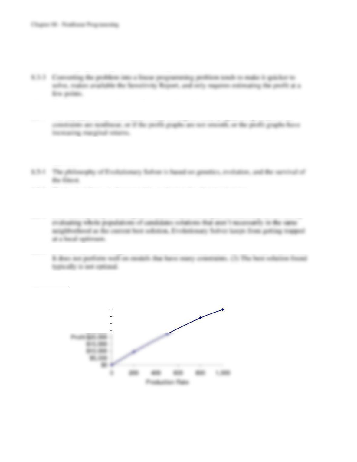
8.1 a)
$0
$5,000
$10,000
$15,000
$20,000
$25,000
$30,000
$35,000
$40,000
0 200 400 600 800 1,000
Production Rate
Profit
b) The proportionality assumption seems to be satisfied reasonably well for this product.
8-4
Case 2
$0
$10
$20
$30
$40
$50
0 1 2 3 4 5
Level of Activity
Profit
Case 3
$0
$1
$2
$3
$4
$5
$6
$7
0 1 2 3 4 5
Level of Activity
Profit
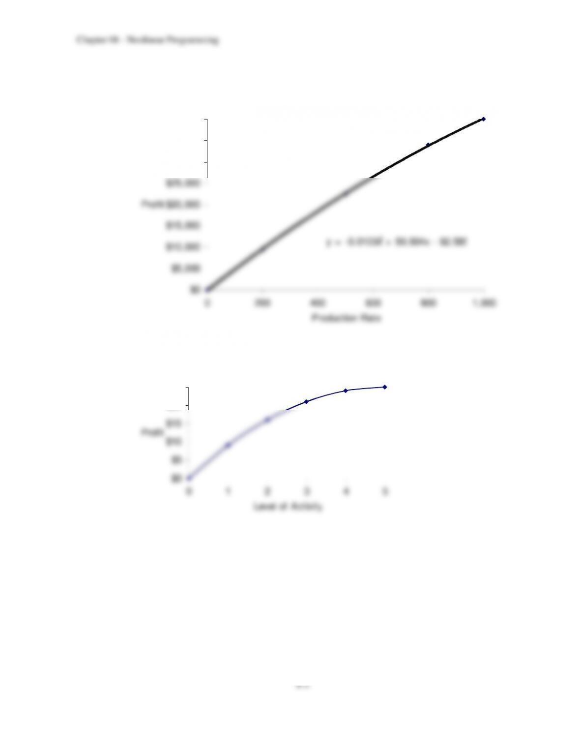
b) Case 1: decreasing marginal returns
Case 2: increasing marginal returns
Case 3: neither increasing nor decreasing marginal returns
8-7
8.4 a)
Production Rate
Actual Profit/Day
Estimated Profit/Day
(P = $100R – $5R2)
Error
0
$0
$0
$0
1
$95
$95
$0
2
$184
$180
$4
3
$255
$255
$0
4
$320
$320
$0
b)
Production Rate
Actual Profit/Day
Estimated Profit/Day
(P = $104R – $6R2)
Error
0
$0
$0
$0
1
$95
$98
$3
2
$184
$184
$0
3
$255
$258
$3
4
$320
$320
$0
c) The quadratic function $100R – 5R2 provides a slightly better fit to all the data.
8.5 In 1995, a number of factors including increased competition, the lack of quantitative tools
to support financial advices and the introduction of new regulations compelled Bank
Hapoalim to review its investment advisory process. Consequently, the Opti- Money
system was developed as a tool to offer systematic financial advice. The underlying
mathematical model is a constrained nonlinear program with continuous or discontinuous
8-8
8.6 a)
3
4
5
6
7
8
9
10
11
12
13
14
15
16
17
18
19
20
21
22
23
24
25
B C D E F G H
Stock 1 Stock 2 Stock 3
Expected Return 21% 30% 8%
Risk (Stand. Dev.) 25% 45% 5%
Jo in t Risk (Covar.) Stock 1 Stock 2 Stock 3
Stock 1 0.040 -0.005
Stock 2 -0.010
Stock 3
Stock 1 Stock 2 Stock 3 Total
Portfolio 69.7% 10.3% 20.0% 100% = 100%
<=
20%
Minimum
Expected
Portfolio Retu rn
Expected Return 19.3% >= 18.0%
Risk (Variance) 0.0365
Risk (Stand. Dev.) 19.1%
The expected return increases by 1.3% and the risk (standard deviation) increases by
about 3.7%.
8-9
b)
3
4
5
6
7
8
9
10
11
12
13
14
15
16
17
18
19
20
21
22
23
24
25
B C D E F G H
Stock 1 Stock 2 Stock 3
Expected Return 21% 30% 8%
Risk (Stand. Dev.) 25% 45% 5%
Jo in t Risk (Covar.) Stock 1 Stock 2 Stock 3
Stock 1 0.040 -0.005
Stock 2 -0.010
Stock 3
Stock 1 Stock 2 Stock 3 Total
Portfolio 87.8% 12.2% 0.0% 100% = 100%
<=
0%
Minimum
Expected
Portfolio Retu rn
Expected Return 22.1% >= 18.0%
Risk (Variance) 0.0598
Risk (Stand. Dev.) 24.4%
The expected return increases by 4.1% and the risk (standard deviation) increases by
about 9%.
c)
27
28
29
30
31
32
33
34
35
36
37
38
39
40
B C D E F G
Risk Expected
Max Stock 3 Stock 1 Stock 2 Stock 3 (St. Dev.) Return
87.8% 12.2% 0.0% 24.4% 22.1%
0% 87.8% 12.2% 0.0% 24.4% 22.1%
5% 83.3% 11.7% 5.0% 23.1% 21.4%
10% 78.8% 11.2% 10.0% 21.8% 20.7%
15% 74.3% 10.7% 15.0% 20.4% 20.0%
20% 69.7% 10.3% 20.0% 19.1% 19.3%
25% 65.2% 9.8% 25.0% 17.8% 18.6%
30% 60.0% 10.0% 30.0% 16.5% 18.0%
35% 47.8% 17.2% 35.0% 15.6% 18.0%
40% 40.2% 21.7% 38.1% 15.4% 18.0%
45% 40.2% 21.7% 38.1% 15.4% 18.0%
50% 40.2% 21.7% 38.1% 15.4% 18.0%
8.7 a) Let S1 = percentage of portfolio to invest in stock 1.
8-10
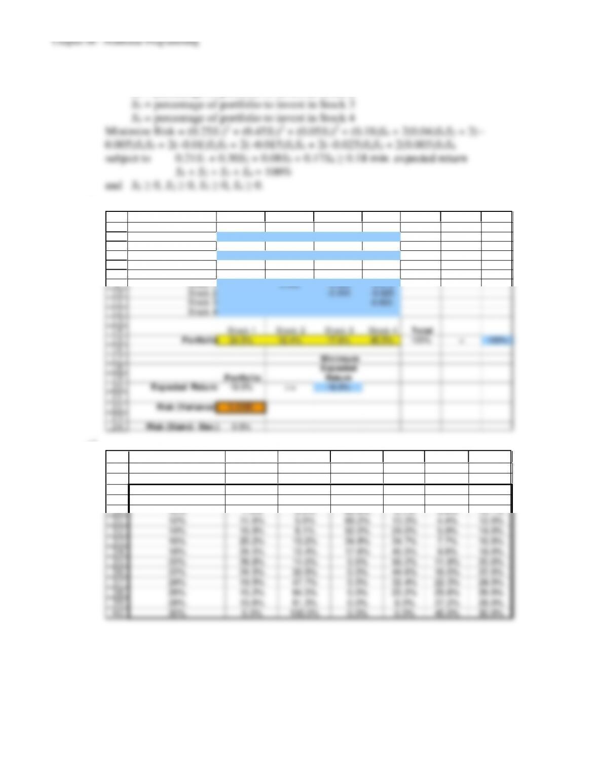
b & c) Minimum acceptable expected profit = $13,000
1
2
3
4
5
6
7
8
9
10
11
12
13
14
15
16
A B C D E F
Stock 1 Stock 2
Expected Profit (on $50,000) $12,500 $20,000
Risk (Stand. Dev. for $50,000) $5,000 $30,000
Stock 1 Stock 2 Total
Portfolio (% of $50,000) 93.3% 6.7% 100% <= 100%
$46,667 $3,333
Minimum
Expected
Portfolio Profit
Expected Profit $13,000 >= $13,000
Risk (Variance) $25,777,778
Risk (Stand. Dev.) $5,077
1
2
3
4
5
6
7
8
9
10
11
12
13
14
15
16
A B C D E F
Stock 1 Stock 2
Expected Profit (on $50,000) $12,500 $20,000
Risk (Stand. Dev. for $50,000) $5,000 $30,000
Stock 1 Stock 2 Total
Portfolio (% of $50,000) 66.7% 33.3% 100% <= 100%
$33,333 $16,667
Minimum
Expected
Portfolio Profit
Expected Profit $15,000 >= $15,000
Risk (Variance) $111,111,111
Risk (Stand. Dev.) $10,541
8-12
8.8 a) Let S1 = percentage of portfolio to invest in Stock 1
S2 = percentage of portfolio to invest in Stock 2
b)
3
4
5
6
7
8
9
10
11
12
13
14
15
16
17
18
19
20
21
22
23
24
B C D E F G H I
Stock 1 Stock 2 Stock 3 Stock 4
Expected Return 21% 30% 8% 17%
Risk (Stand . Dev.) 25% 45% 5% 18%
Joint Risk (Covar.) Stock 1 Stock 2 Stock 3 Stock 4
Stock 1 0.040 -0.005 –0.015
Stock 2 -0.010 –0.025
Stock 3 0.003
Stock 4
Stock 1 Stock 2 Stock 3 Stock 4 Total
Portfolio 24.5% 12.4% 17.6% 45.5% 100% = 100%
Minimum
Expected
Portfolio Return
Expected Return 18.0% >= 18.0%
Risk (Variance) 0.0095
Risk (Stand . Dev.) 9.8%
c)
26
27
28
29
30
31
32
33
34
35
36
37
38
39
40
B C D E F G H
Minimum Risk Expected
Expected Return Stock 1 Stock 2 Stock 3 Stock 4 (St. Dev.) Return
24.5% 12.4% 17.6% 45.5% 9.8% 18.0%
8% 7.5% 3.9% 85.6% 3.1% 3.8% 10.1%
10% 7.5% 3.9% 85.6% 3.1% 3.8% 10.1%
12% 11.6% 5.9% 69.2% 13.3% 4.4% 12.0%
14% 15.9% 8.1% 52.0% 24.0% 5.9% 14.0%
16% 20.2% 10.2% 34.8% 34.7% 7.7% 16.0%
18% 24.5% 12.4% 17.6% 45.5% 9.8% 18.0%
20% 28.8% 14.5% 0.5% 56.2% 11.9% 20.0%
22% 24.5% 30.9% 0.0% 44.6% 16.0% 22.0%
24% 19.9% 47.7% 0.0% 32.4% 22.3% 24.0%
26% 15.2% 64.5% 0.0% 20.2% 29.6% 26.0%
28% 10.6% 81.3% 0.0% 8.0% 37.2% 28.0%
30% 0.0% 100.0% 0.0% 0.0% 45.0% 30.0%
8-14
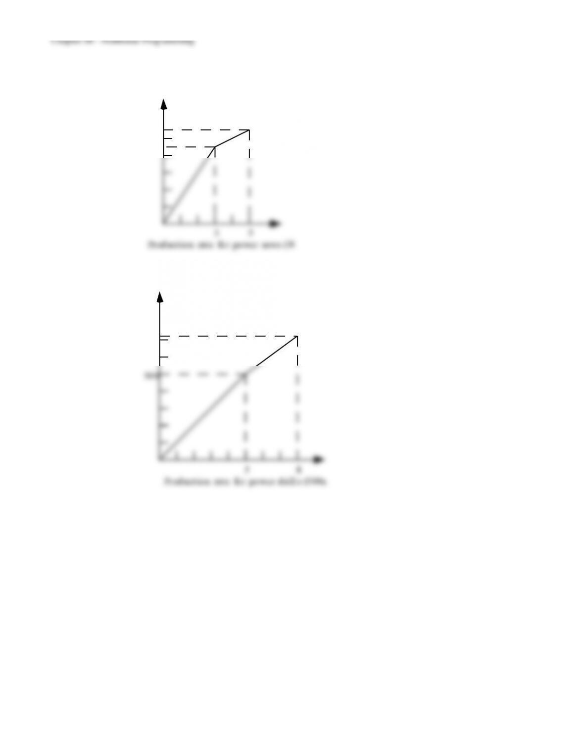
8.10 a) The profit graph for power saws is shown below:
Prod uct ion rat e for po wer saws (00
Monthl y
Profit ($0 00)
3 5
450
550
The profit graph for power drills is shown below:
Prod uct ion rat e fo r power d ri ll s (000s
Monthl y
Profit ($0 00)
85
725
500
8-15
b)
1
2
3
4
5
6
7
8
9
10
11
12
13
14
15
A B C D E F
Unit Profit Power Saws Power Drills
Regular Time $150 $100
Overtime $50 $75
Total
Used Available
Power Supplies 1 1 10,000 <= 10,000
Gear Assemblies 2 1 13,000 <= 15,000
Power Saws Power Drills Power Saws Power Drills
Regular Time 3,000 5,000 <= 3,000 5,000
Overtime 0 2,000 <= 2,000 3,000
Total 3,000 7,000
Total Profit
$1,100,000
Units Produced
Maximum
Used per Unit Produced
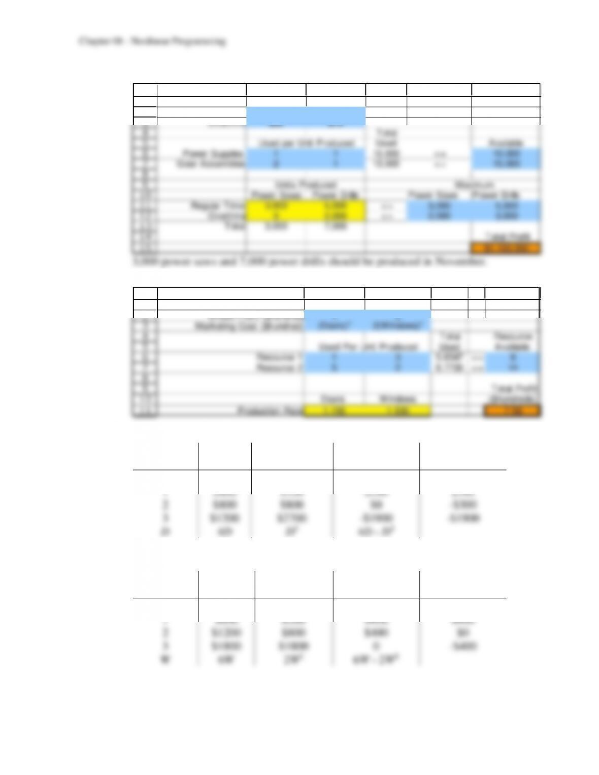
3,000 power saws and 7,000 power drills should be produced in November.
8.11 a)
1
2
3
4
5
6
7
8
9
10
11
A B C D E F
Unit Profit Doors W indows
Gross Profit ($hundred) 4 6
Marketing Cost ($hundred) (Doors)32(W indows)2
Total Resource
Used Available
Resource 1 1 3 5.6547 <= 8
Resource 2 5 2 8.7735 <= 14
Total Profit
Doors Windows ($hundreds)
Production Rate 1.155 1.500 7.58
Used Per Unit Produced
b) Profit data for doors when marketing costs are considered:
Production
Rate
Gross
Profit
Marketing
Cost
Net Profit
Incremental
Net Profit
0
0
0
0
—
1
$400
$100
$300
$300
2
$800
$800
$0
-$300
3
$1200
$2700
-$1900
-$1900
D
4D
D3
4D – D3
Profit data for windows when marketing costs are considered:
Production
Rate
Gross
Profit
Marketing
Cost
Net Profit
Incremental
Net Profit
0
0
0
0
—
1
$600
$200
$400
$400
2
$1200
$800
$400
$0
3
$1800
$1800
0
-$400
W
6W
2W2
6W – 2W2
8-16
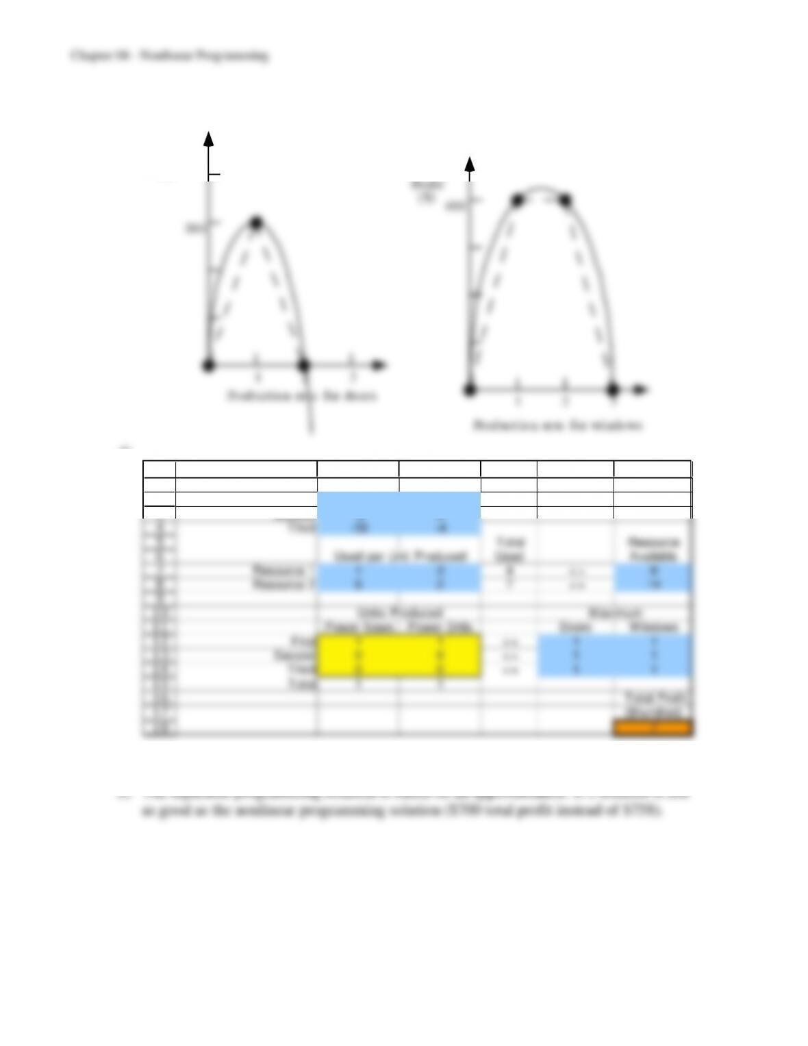
c) The profit graphs for doors and windows are shown below:
Product ion ra te for doors
W eekly
Profit
($)
3
300
1 2
Prod uct io n ra te for wi ndows
W eek ly
Profit
($)
3
400
1 2
d)
1
2
3
4
5
6
7
8
9
10
11
12
13
14
15
16
17
18
A B C D E F
Unit Profit ($hundred) Doors Windows
First 3 4
Second -3 0
Third -19 -4
Total Resource
Used Available
Resource 1 1 3 4 <= 8
Resource 2 5 2 7 <= 14
Power Saws Power Drills Doors Windows
First 1 1 <= 1 1
Second 0 0 <= 1 1
Third 0 0 <= 1 1
Total 1 1
Total Profit
($hundred)
7
Units Produced
Maximum
Used per Unit Produced
Dorwyn should produce 1 door and 1 window.
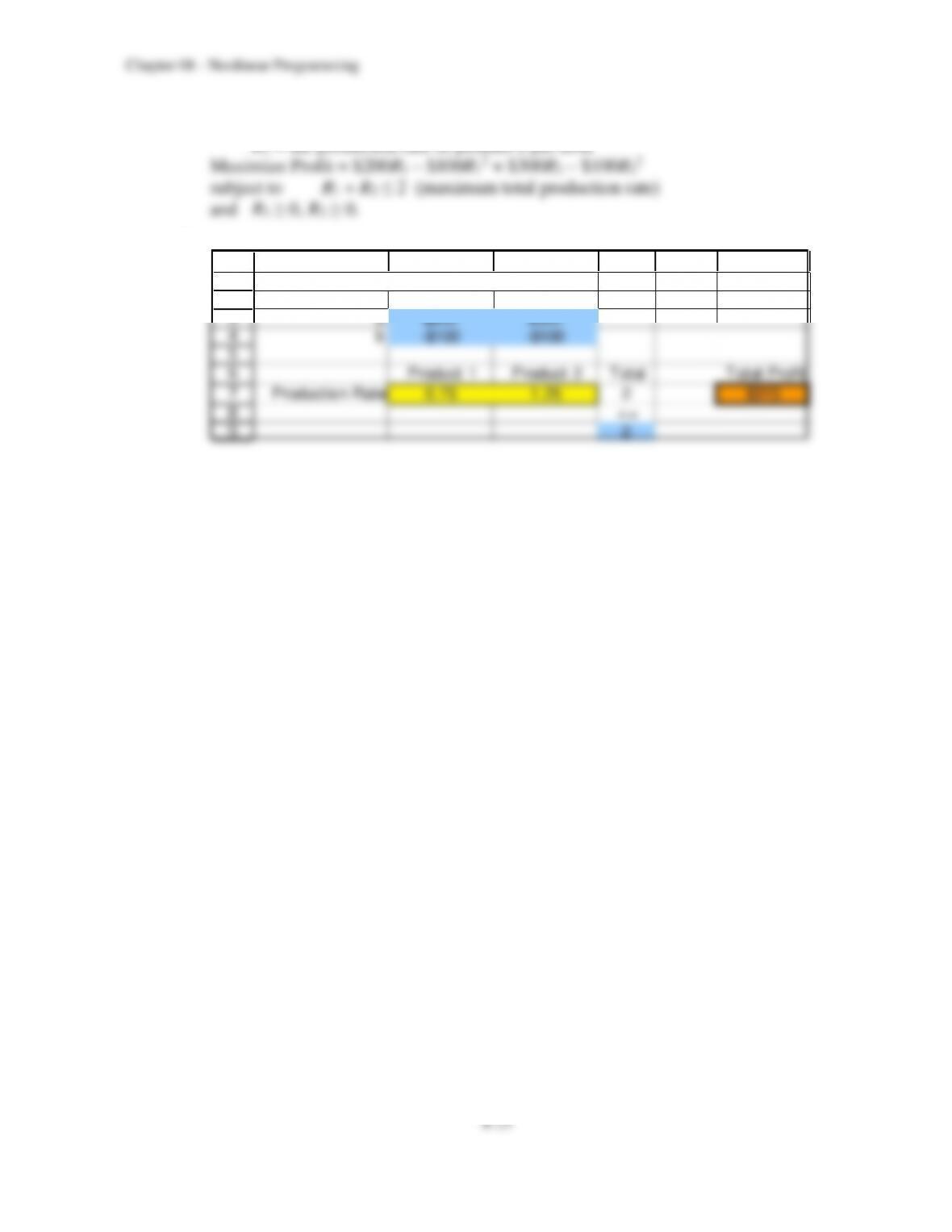
8.13 The profit graph for product 1 is shown below:
Product ion of produc t 1
Profit
2
10
5
22
The profit graph for product 2 is shown below:
Product i on of produc t
Profit
3
12
4
13