7-1
Chapter 7 Using Binary Integer Programming to Deal with Yes-or-No
Decisions
Review Questions
7.1-1 The decisions are 1) whether to build a factory in Los Angeles, 2) whether to build a
7.1-2 Binary decision variables are appropriate because there are only two alternatives, choose
yes or choose no.
7.1-4 The mutually exclusive alternatives are to build a warehouse in Los Angeles or build a
7.1-5 The contingent decisions are the decisions to build a warehouse. The forms of these
constraints are x3 ≤ x1 and x4 ≤ x2.
7.1-6 The amount of capital being made available to these investments ($10 million) is a
managerial decision on which sensitivity analysis needs to be performed.
7.2-2 The projects under consideration are yes-or-no projects that must be done in their entirety
or not at all.
7.2-3 The objective is to select the projects to approve that will maximize the expected total
profit.
7.3-2 Fire stations, police stations, or ambulance centers are examples of types of emergency
services faciliteis for which sites may need to be selected.
7.3-3 The objective is to minimize the total cost of the fire stations that will satisfy the City
Council’s new policy on response times.
7-2
7.4-1 The crew scheduling problem that is encountered by companies in the travel industry is
7.4-2 The yes-or-no decisions are whether a particular sequence should be assigned to a crew.
7.4-3 The mathematical form of the constraint is x1 + x4 + x7 + x10 ≥ 1. This constraint says that
7.5-1 In a mixed BIP problem, only some of the decision variables are binary variables.
7.5-2 The net profit for either product is no longer directly proportional to the number of units
7.5-4 The setup cost required to start producing a product caused the optimal solution to change
so that only one of the products is produced, and hence only one setup cost is incurred.
Problems
7.1 Prior to this study, Waste Management, Inc. (WM) encountered several operational
inefficiencies concerning the routing of its trucks. The routes served by different trucks had
routes with minimum number of vehicles and travel time, maximum visual attractiveness
and a balanced workload. First, a network with nodes that represent actual stops, landfills,
lunch break and the depot is constructed. The binary variables xijk refer to whether arc (i, j)
is included in the route of vehicle k or not. The integer variables Nk denote the number of
route includes a lunch break. An iterative two-phase algorithm enhanced with
metaheuristics is employed to solve the problem.
7-3
Financial benefits of this study include savings of approximately $18 million in 2003 and
estimated savings of $44 million in 2004. WM expects to save more and to increase its
cash flow by $648 million over a five-year interval. The savings in operational costs over
quickly, since they know the routes of the vehicles. As a result, WM provides a more
reliable customer service. Operational efficiency also affected the environment and the
employees positively. Emissions and noise are reduced. Finally, the benefits from this
study led WM to exploit operations research techniques in other operational areas, too.
7.2 a) Let FLA = 1 if build a factory in Los Angeles; 0 otherwise
FSF = 1 if build a factory in San Francisco; 0 otherwise
Maximize NPV ($million) = 9FLA + 5FSF + 7FSD + 6WLA + 4WSF + 5WSD
subject to 6FLA + 3FSF + 4FSD + 5WLA + 2WSF + 3WSD ≤ $10 million (Capital)
WLA + WSF + WSD ≤ 1 warehouse
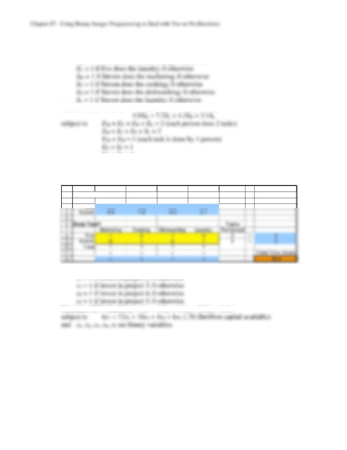
b)
3
4
5
6
7
8
9
10
11
12
13
14
15
16
17
18
19
20
B C D E F G H
NPV ($millions) Los Angeles San Francisco San Diego
W arehouse 6 4 5
Factory 8 5 7
Cap ital Required
($millions) Los Angeles San Francisco San Diego
W arehouse 5 2 3 Capital Capital
Spent Available
Factory 6 3 4 10 <= 10
Total Maximum
Build? Los Angeles San Francisco San Diego W arehouses W arehouses
W arehouse 0 0 1 1 <= 1
<= <= <=
Factory 0 1 1
Total NPV ($millions) 17
7-4
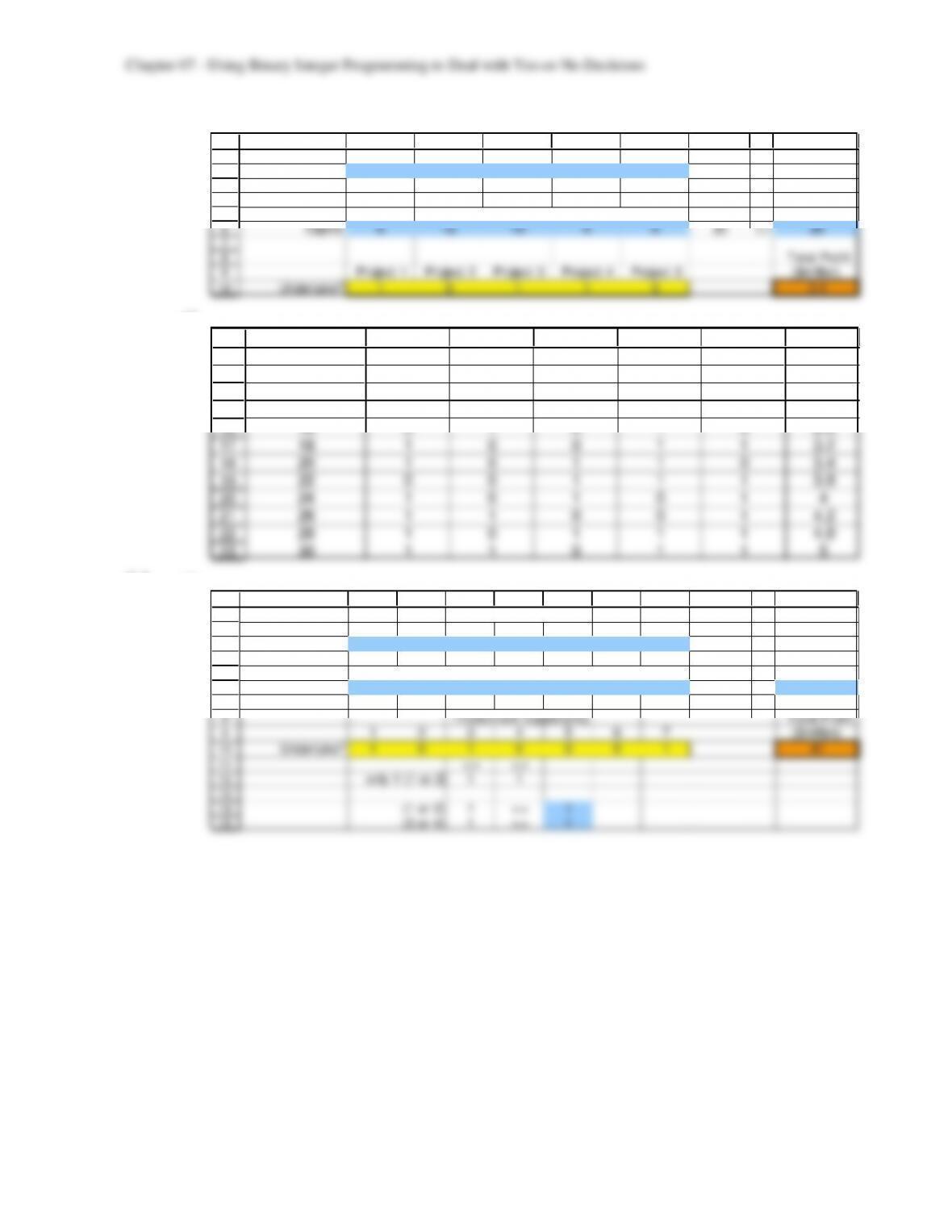
7.3 a) Let EM = 1 if Eve does the marketing; 0 otherwise
EC = 1 if Eve does the cooking; 0 otherwise
ED = 1 if Eve does the dishwashing; 0 otherwise
Minimize Time (hours) = 4.5EM + 7.8EC + 3.6ED + 2.9EL +
ED + SD = 1
EL + SL = 1
and EM, EC, ED, EL, SM, SC, SD, SL are binary variables.
b)
1
2
3
4
5
6
7
8
9
10
11
12
A B C D E F G H
Time Needed (hours)
Marketing Cooking Dishwashing Laundry
Eve 4.5 7.8 3.6 2.9
Steven 4.9 7.2 4.3 3.1
Does Task? Tasks
Marketing Cooking Dishwashing Laundry Performed
Eve 1 0 1 0 2 = 2
Steven 0 1 0 1 2 = 2
Total 1 1 1 1
= = = = Total Time (hours)
1 1 1 1 18.4
7.4 a) Let x1 = 1 if invest in project 1; 0 otherwise
Maximize NPV ($million) = 1x1 + 1.8x2 + 1.6x3 + 0.8x4 + 1.4x5
7-5
b)
1
2
3
4
5
6
7
8
9
10
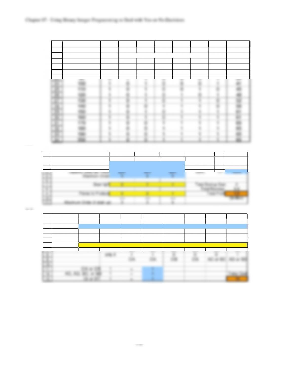
A B C D E F G H I
Project 1 Project 2 Project 3 Project 4 Project 5
Estimated Profit 1 1.8 1.6 0.8 1.4
($million) Capital Capital
Spent Available
Capital Required for Project ($million) ($million) ($million)
Capital 6 12 10 4 8 20 <= 20
Total Profit
Project 1 Project 2 Project 3 Project 4 Project 5 ($million)
Undertake? 1 0 1 1 0 3.4
c)
12
13
14
15
16
17
18
19
20
21
22
23
A B C D E F G
Capital Total
Available Undertake? Profit
($million) Project 1 Project 2 Project 3 Project 4 Project 5 ($million)
1 0 1 1 0 3.4
16 0 1 0 1 0 2.6
18 1 0 0 1 1 3.2
20 1 0 1 1 0 3.4
22 0 0 1 1 1 3.8
24 1 0 1 0 1 4
26 1 1 0 0 1 4.2
28 1 0 1 1 1 4.8
30 1 1 0 1 1 5
7.5 a)
1
2
3
4
5
6
7
8
9
10
11
12
13
14
15
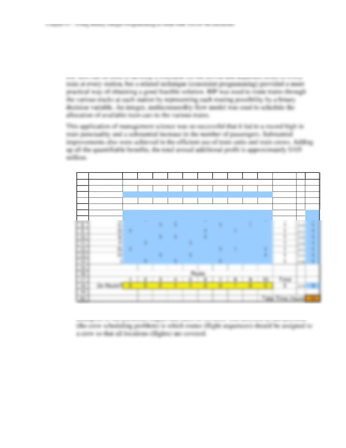
A B C D E F G H I J K
Investment O pportunity
1 2 3 4 5 6 7
Estimated Profit 17 10 15 19 713 9
($million) Capital Capital
Capital Required for Investment Opportunity ($million) Spent Available
Capital 43 28 34 48 17 32 23 100 <= 100
Investment O pportunity Total Profit
1 2 3 4 5 6 7 ($million)
Undertake? 1 0 1 0 0 0 1 41
<= <=
only if (1 or 2) 1 1
(1 or 2) 1 <= 1
(3 or 4) 1 <= 1
7-7
7.8 Netherlands Railways used BIP and related techniques in a variety of ways in this massive
application of management science. For example, a BIP model similar to the one illustrated
in Section 7.4 (but vastly larger) was used to schedule the assignment of crews (with a train
driver and a number of conductors in each crew) for each of the 5,500 trains in the system.
7.9 a)
1
2
3
4
5
6
7
8
9
10
11
12
13
14
15
16
17
18
19
20
A B C D E F G H I J K L M N
1 2 3 4 5 6 7 8 9 10
Time (hours) 6 4 7 5 4 6 5 3 7 6
Total on
Location Route
A 1 1 1 1 >= 1
B 1 1 1 1 1 1 >= 1
C 1 1 1 1 1 >= 1
D 1 1 1 1 >= 1
E 1 1 1 1 >= 1
F 1 1 1 >= 1
G 1 1 1 1 1 >= 1
H 1 1 1 1 >= 1
I 1 1 1 1 >= 1
1 2 3 4 5 6 7 8 9 10 Total
Do Route? 0 0 0 1 1 0 0 1 0 0 3 <= 3
Total Time (hours) 12
Route
Route
Delivery Location on Route?
b) The delivery routes are analagous to the flight sequences, and the locations are
analagous to the particular flights that must be covered. The decision in this problem
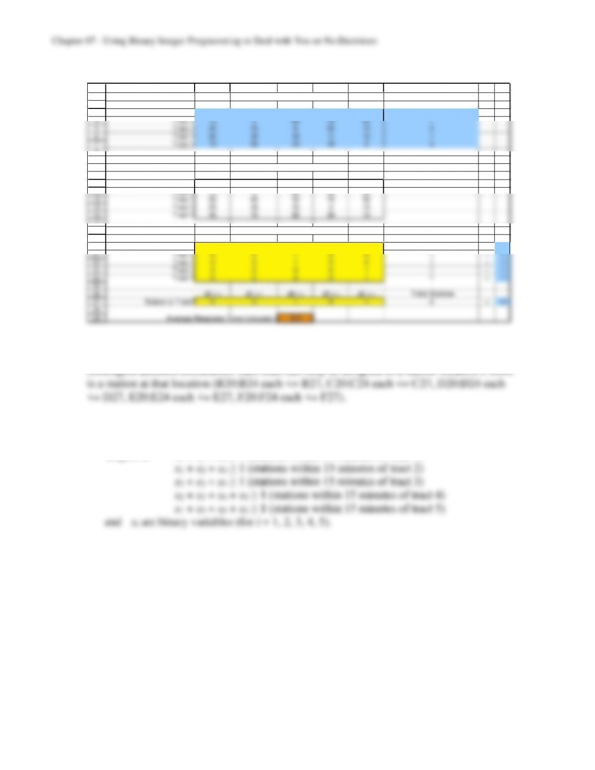
7-8
7.10
1
2
3
4
5
6
7
8
9
10
11
12
13
14
15
16
17
18
19
20
21
22
23
24
25
26
27
28
29
A B C D E F G H I
Response Station Location Avg. Emergencies
Time (min) Tract 1 Tract 2 Tract 3 Tract 4 Tract 5 per Day
Tract 1 5 20 15 25 10 2
Tract 2 12 420 15 25 1
Tract 3 30 15 625 15 3
Tract 4 20 10 15 412 1
Tract 5 15 25 12 10 5 3
Average Total Station Location
Response Time Tract 1 Tract 2 T ract 3 Tract 4 T ract 5
Tract 1 10 40 30 50 20
Tract 2 12 420 15 25
Tract 3 90 45 18 75 45
Tract 4 20 10 15 412
Tract 5 45 75 36 30 15
Tract Assigned to Station? Total Number of
Tract 1 Tract 2 T ract 3 Tract 4 Tract 5 Stations Assigned to Tract
Tract 1 0 0 0 0 1 1 = 1
Tract 2 0 0 1 0 0 1 = 1
Tract 3 0 0 1 0 0 1 = 1
Tract 4 0 0 0 0 1 1 = 1
Tract 5 0 0 0 0 1 1 = 1
all < = all <= all < = all < = all < = Total Stations
Station in Tract? 0 0 1 0 1 2 = 2
Average Response Time (minutes) = 8.5
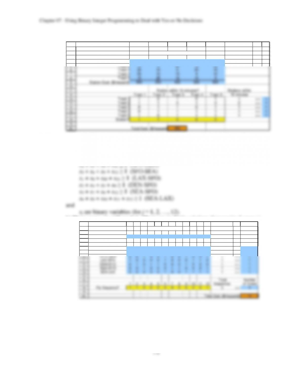
The six equality constraints (total stations = 2; one station assigned to each tract)
correspond to mutually exclusive alternatives. In addition, there are the following
7.11 a) Let xi = 1 if a station is located in tract i; 0 otherwise (for i = 1, 2, 3, 4, 5)
Minimize Cost ($thousand) = 200x1 + 250x2 + 400x3 + 300x4 + 500x5
subject to x1 + x3 + x5 ≥ 1 (stations within 15 minutes of tract 1)
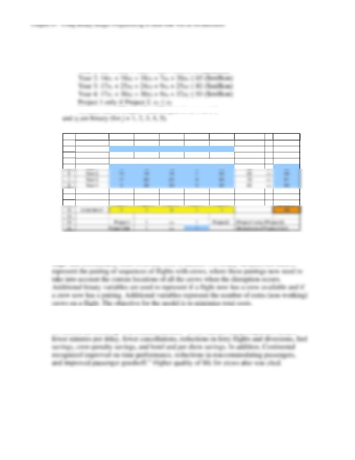
7-10
7.13 a) Let xj = 1 if project j is done; 0 otherwise (for j = 1, 2, 3, 4, 5).
Maximize Total NPV = 12x1 + 15x2 + 20x3 + 9x4 + 23x5 ($million)
subject to
Year 1: 8x1 + 10x2 + 12x3 + 4x4 + 14x5 ≤ 40 ($million)
At most one of Project 3 and Project 4: x3 + x4 ≤ 1
b)
1
2
3
4
5
6
7
8
9
10
11
12
13
14
15
A B C D E F G H I
Project 1 Project 2 Project 3 Project 4 Project 5
NPV ($million) 12 15 20 923
Cumulative Cumulative
Cumulative Cash Outflow Required ($million) Outflow Available
Year 1 8 10 12 414 36 <= 40
Year 2 14 18 18 720 59 <= 65
Year 3 17 25 24 925 76 <= 81
Year 4 0 30 30 032 62 <= 93
Total NPV
Project 1 Project 2 Project 3 Project 4 Project 5 ($million)
Undertake? 1 1 0 1 1 59
Project 1 1 <= 1 Project 2 (Project 1 only if Project 2)
Project 3&4 1 <= 1 (At most one of Project 3 & 4)
7.14 A management science team at Continental Airlines developed a massive BIP model for
quickly reassigning crews to flights as soon as disruptions cause flight delays and
cancellations. The model is similar to the one illustrated in Section 7.4, except massively
larger and considerably more involved. Like in Section 7.4, binary variables are used to
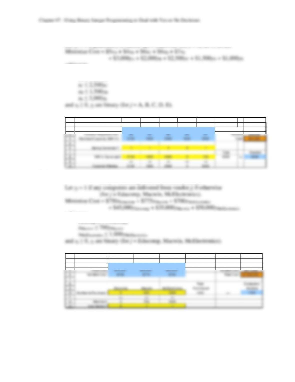
The new system for quickly reassigning crews to flights based on this mixed BIP model
provided faster and more efficient recovery solutions than Continental’s previous system.
As cited in the article [p. 14], benefits included “fewer enroute and predeparture delays,
During its first year of use (which included dealing with the disruptions caused by the
terrorist attacks on September 11, 2001), the new system led to savings of approximately
$40 million. The use of the system was expected to grow considerably in subsequent years
7.15 a) Let xj = megawatt-hours generated at generator j (for j = A, B, C, D, E).
Let yj = 1 if generator j is started up; 0 otherwise (for j = A, B, C, D, E).
subject to
xA ≤ 2,100yA
xB ≤ 1,800yB
b)
1
2
3
4
5
6
7
8
9
10
A B C D E F G H I
A B C D E Cost
Fixed Startup Cost $3,000 $2,000 $2,500 $1,500 $1,000 Startup $8,500
Cost per Megawatt–hour $5 $4 $6 $6 $7 Variable $33,400
Maximum Capacity (MW–hr) 2100 1800 2500 1500 3000 Total $41,900
Startup Generator? 1 1 1 0 1
Total Needed
MW-hr Generated 2100 1800 2500 0 100 6500 >= 6500
<= <= <= <= <=
Capacity if Startup 2100 1800 2500 0 3000
7.16 a) Let xj = number of computers purchased from vendor j
(for j = Educomp, Macwin, McElectronics).
subject to
b)
3
4
5
6
7
8
9
10
11
12
13
B C D E F G H
Educomp Macwin McElectronics
Capacity 700 700 1000 Fixed Cost $85,000
Fixed Cost $45,000 $35,000 $50,000 Variable Cost $971,250
Variable Cost $750 $775 $700 Total Cost $1,056,250
Total Computers
Educomp Macwin McElectronics Purchased Needed
Number to Purchase 0 350 1000 1350 >= 1350
<= <= <=
Maximum 0 700 1000
Use Vendor? 0 1 1
7.18 a)
1
2
3
4
5
6
7
8
9
10
11
12
13
14
15
16
17
18
19
20
21
22
23
24
25
26
27
28
29
30
31
A B C D E F G H I J K L
Distribution Problem (part a)
Nashville San J ose Hous ton Production
Shipping Cost Warehouse Warehouse Warehouse Cost Capacity Costs
Atlanta Plant $30 $40 $50 $208 200 Shipping(P––>WH) $20,000
KC Plant $25 $45 $40 $214 300 Shipping(WH––>C) $12,875
Aberdeen Plant $45 $30 $55 $215 300 Production (P) $143,050
Austin Plant $30 $50 $30 $210 400 Variable (WH) $3,125
Total $179,050
Nashville San J ose Hous ton Total
Shipments Warehouse Warehouse Warehouse Produced Capacity
Atlanta Plant 200 0 0 200 <= 200
KC Plant 50 0 0 50 <= 300
Aberdeen Plant 0 300 0 300 <= 300
Austin Plant 0 0 125 125 <= 400
Total 250 300 125
Shipped
Variable
Shipping Cost Sears Best Buy Fry ‘s Comp USA Office Max Cost Capacity
Nashville WH $40 $45 $30 $25 $20 $4 300
San J ose WH $15 $50 $25 $15 $40 $5 500
Hous ton WH $50 $35 $15 $40 $50 $5 500
Total Total
Shipments Sears Best Buy Fry‘s Comp USA Office Max Shipped Out Shipped In Capacity
Nashville WH 0 0 0 100 150 250 <= 250 <= 300
San J ose WH 100 0 0 200 0 300 <= 300 <= 500
Hous ton WH 0 50 75 0 0 125 <= 125 <= 500
Total 100 50 75 300 150
>= >= >= >= >=
Demand 100 50 75 300 150
b)
1
2
3
4
5
6
7
8
9
10
11
12
13
14
15
16
17
18
19
20
21
22
23
24
25
26
27
28
29
30
31
A B C D E F G H I J K L M N
Distribution Problem (part b)
Nashville San J ose Hous ton Production Fixed Costs
Shipping Cost Warehouse Warehouse Warehouse Cost Capacity Cost Shipping(P––>WH) $21,750
Atlanta Plant $30 $40 $50 $208 200 $8,000 Shipping(WH––>C) $13,750
KC Plant $25 $45 $40 $214 300 $9,000 Production (P) $143,250
Aberdeen Plant $45 $30 $55 $215 300 $9,000 Variable (WH) $3,075
Austin Plant $30 $50 $30 $210 400 $10,000 Fixed (P) $19,000
Fixed (WH) $9,000
Nashville San J ose Hous ton Total Total $209,825
Shipments Warehouse Warehouse Warehouse Produced Capacity Open?
Atlanta Plant 0 0 0 0 <= 0 0
KC Plant 0 0 0 0 <= 0 0
Aberdeen Plant 0 300 0 300 <= 300 1
Austin Plant 300 75 0 375 <= 400 1
Total 300 375 0
Shipped
Variable Fixed
Shipping Cost Sears Bes t Buy Fry‘s Comp USA Office Max Cost Capacity Cost
Nashville WH $40 $45 $30 $25 $20 $4 300 $4,000
San J ose WH $15 $50 $25 $15 $40 $5 500 $5,000
Hous ton WH $50 $35 $15 $40 $50 $5 500 $5,000
Total Total
Shipments Sears Best Buy Fry‘s Comp USA Office Max Shipped Out Shipped In Capacity Open?
Nashville WH 0 50 75 25 150 300 <= 300 <= 300 1
San J ose WH 100 0 0 275 0 375 <= 375 <= 500 1
Hous ton WH 0 0 0 0 0 0 <= 0<= 0 0
Total 100 50 75 300 150
>= >= >= >= >=
Demand 100 50 75 300 150
7-14
Cases
7.1 a) We want to maximize the number of pieces displayed in the exhibit. For each piece,
we therefore need to decide whether or not we should display the piece. Each piece
becomes a binary decision variable. The decision variable is assigned 1 if we want to
Artistic Constraints Imposed by Ash
Ash imposes the following constraints that depend upon the type of art that is
displayed. The constraints are as follows:
2. Ash wants at least one wire-mesh sculpture displayed if a computer-generated
drawing is displayed. We have three wire-mesh sculptures available and two
computer-generated drawings available. Thus, if we include either one or two
3. Ash wants at least one computer-generated drawing displayed if a wire-mesh
sculpture is displayed. We have two computer-generated drawings available and three
wire-mesh sculptures available. Thus, if we include one, two, or three wire-mesh
4. Ash wants at least one photo-realistic painting displayed. We have three photo-
realistic paintings available: “Storefront Window” by David Lyman, “Harley” by
5. Ash wants at least one cubist painting displayed. We have three cubist paintings
available: “Rick II” by Rick Rawls, “Study of a Violin” by Helen Row, and “Study of