Chapter 06 – Network Optimization Problems
6-19
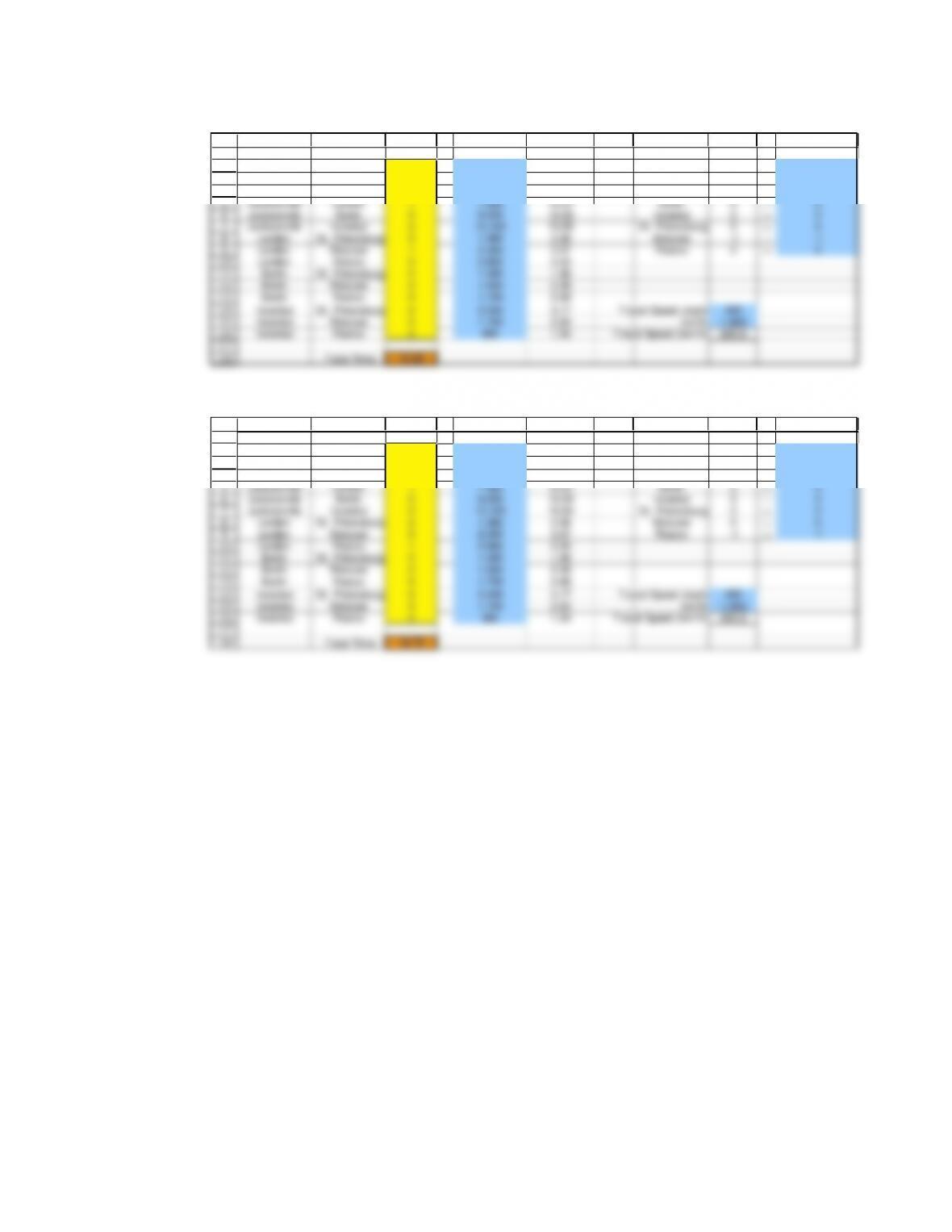
Jacksonville to Moscow:
1
2
3
4
5
6
7
8
9
10
11
12
13
14
15
16
17
18
A B C D E F G H I J K
From To O n Route Distance (km) Time (hou rs) Node Net F lo w Supply/Demand
Boston London 0 6,200 9.63 Boston 0 = 0
Boston Berlin 0 7,250 11.26 Jacksonville 1 = 1
Boston Istanbul 0 8,300 12.90 London 0 = 0
Jacksonville London 1 7,900 12.27 Berlin 0 = 0
Jacksonville Berlin 0 9,200 14.29 Istanbul 0 = 0
Jacksonville Istanbul 0 10,100 15.69 St. Petersburg 0 = 0
London St. Petersburg 0 1,980 3.08 Moscow -1 =-1
London Moscow 1 2,300 3.57 Rostov 0 = 0
London Rostov 0 2,860 4.44
Berlin St. Petersburg 0 1,280 1.99
Berlin Moscow 0 1,600 2.49
Berlin Rostov 0 1,730 2.69
Istanbul St. Petersburg 0 2,040 3.17 Travel Speed (mph) 400
Istanbul Moscow 0 1,700 2.64 km/hr 1.609
Istanbul Rostov 0 990 1.54 Travel Speed (km/hr) 643.6
Total Time 15.85
Jacksonville to Rostov:
1
2
3
4
5
6
7
8
9
10
11
12
13
14
15
16
17
18
A B C D E F G H I J K
From To O n Route Distance (km) Time (hou rs) Node Net F lo w Supply/Demand
Boston London 0 6,200 9.63 Boston 0 = 0
Boston Berlin 0 7,250 11.26 Jacksonville 1 = 1
Boston Istanbul 0 8,300 12.90 London 0 = 0
Jacksonville London 1 7,900 12.27 Berlin 0 = 0
Jacksonville Berlin 0 9,200 14.29 Istanbul 0 = 0
Jacksonville Istanbul 0 10,100 15.69 St. Petersburg 0 = 0
London St. Petersburg 0 1,980 3.08 Moscow 0 = 0
London Moscow 0 2,300 3.57 Rostov -1 =-1
London Rostov 1 2,860 4.44
Berlin St. Petersburg 0 1,280 1.99
Berlin Moscow 0 1,600 2.49
Berlin Rostov 0 1,730 2.69
Istanbul St. Petersburg 0 2,040 3.17 Travel Speed (mph) 400
Istanbul Moscow 0 1,700 2.64 km/hr 1.609
Istanbul Rostov 0 990 1.54 Travel Speed (km/hr) 643.6
Total Time 16.72
6-20
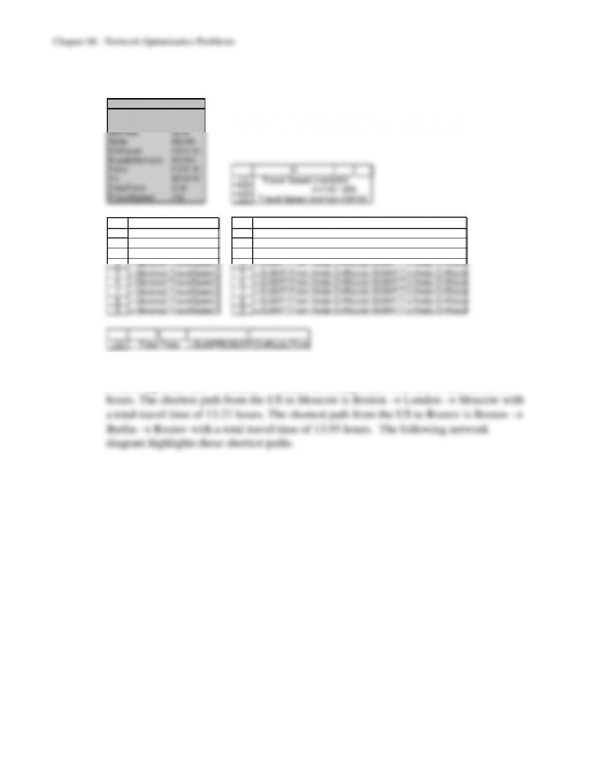
The spreadsheets contain the following formulas:
Rang e Name Cells
Distance E2:E16
From A2:A16
NetF low I2:I9
Node H2:H9
O nRout e C2:C16
SupplyDemand K2:K9
Time F2:F 16
To B2:B16
TotalTime C18
TravelSpeed I16
14
15
16
H I
Travel Speed (mph) 400
km/hr 1.609
Travel Speed (km/hr)= I14*I15
1
2
3
4
5
6
7
8
9
F
Time (hours)
= Dist ance/TravelSpeed
= Dist ance/TravelSpeed
= Dist ance/TravelSpeed
= Dist ance/TravelSpeed
= Dist ance/TravelSpeed
= Dist ance/TravelSpeed
= Dist ance/TravelSpeed
= Dist ance/TravelSpeed
1
2
3
4
5
6
7
8
9
I
Net Flo w
=SUMIF(From,Node,OnRoute)-SUMIF(To,Node,OnRoute
=SUMIF(From,Node,OnRoute)-SUMIF(To,Node,OnRoute
=SUMIF(From,Node,OnRoute)-SUMIF(To,Node,OnRoute
=SUMIF(From,Node,OnRoute)-SUMIF(To,Node,OnRoute
=SUMIF(From,Node,OnRoute)-SUMIF(To,Node,OnRoute
=SUMIF(From,Node,OnRoute)-SUMIF(To,Node,OnRoute
=SUMIF(From,Node,OnRoute)-SUMIF(To,Node,OnRoute
=SUMIF(From,Node,OnRoute)-SUMIF(To,Node,OnRoute
18
B C
Total Time =SUMPRODUCT(OnRoute,Time)
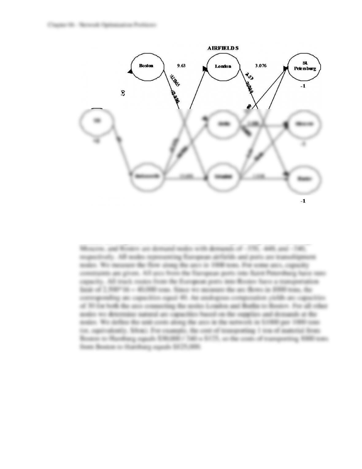
Comparing all six solutions we see that the shortest path from the US to Saint
Petersburg is Boston → London → Saint Petersburg with a total travel time of 12.71
6-21
c) The President must satisfy each Russian city’s military requirements at minimum cost.
Therefore, this problem can be solved as a minimum-cost network flow problem. The
two nodes representing US cities are supply nodes with a supply of 500 each (we
measure all weights in 1000 tons). The three nodes representing Saint Petersburg,
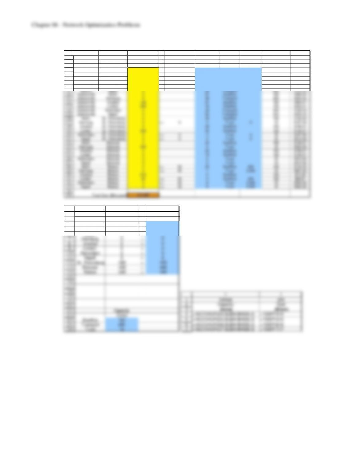
The objective is to satisfy all demands in the network at minimum cost. The following
spreadsheet shows the entire linear programming model.
6-22
1
2
3
4
5
6
7
8
9
10
11
12
13
14
15
16
17
18
19
20
21
22
23
24
25
26
27
28
29
30
31
32
33
34
35
A B C D E F G H I J
Cost per Vehicle Unit
Ship Capacity Vehicle Maximum Capacity Cost
From To (th ou sand tons) (th ousand to n s) ($thousand ) Vehicle Vehicles (to ns) ($/to n )
Boston Berlin 0 50 Starlifter 150 $333.33
Boston Hamburg 440 30 Transport 240 $125.00
Boston Istanbul 60 55 Starlifter 150 $366.67
Boston London 0 45 Starlifter 150 $300.00
Boston Rotterdam 0 30 Transport 240 $125.00
Boston Napoli 0 32 T ransport 240 $133.33
Jacksonville Berlin 0 57 Starlifter 150 $380.00
Jacksonville Hamburg 0 48 Transport 240 $200.00
Jacksonville Istanbul 150 61 Starlifter 150 $406.67
Jacksonville London 350 49 Starlifter 150 $326.67
Jacksonville Rotterdam 0 44 Transport 240 $183.33
Jacksonville Napoli 0 56 Transport 240 $233.33
Berlin St. Petersburg 0 24 Starlifter 150 $160.00
Hamburg St. Petersburg 0 <= 0 3 T ruck 0 16 $187.50
Istanbul St. Petersburg 0 28 Starlifter 150 $186.67
London St. Petersburg 320 22 Starlifter 150 $146.67
Rotterdam St. Petersburg 0 <= 0 3 T ruck 0 16 $187.50
Napoli St. Petersburg 0 <= 0 5 Truck 0 16 $312.50
Berlin Moscow 0 22 Starlifter 150 $146.67
Hamburg Moscow 440 4 Truck 16 $250.00
Istanbul Moscow 0 25 Starlifter 150 $166.67
London Moscow 0 19 Starlifter 150 $126.67
Rotterdam Moscow 0 5 Truck 16 $312.50
Napoli Moscow 0 5 Truck 16 $312.50
Berlin Rostov 0 <= 30 23 Starlifter 200 150 $153.33
Hamburg Rostov 0 <= 40 7 Truck 2,500 16 $437.50
Istanbul Rostov 210 2 Starlifter 150 $13.33
London Rostov 30 <= 30 4 Starlifter 200 150 $26.67
Rotterdam Rostov 0 <= 40 8 Truck 2,500 16 $500.00
Napoli Rostov 0 <= 40 9 T ruck 2,500 16 $562.50
Total Cost ($thousand) 412,867
2
3
4
5
6
7
8
9
10
11
12
13
14
15
16
17
18
19
20
21
22
23
24
25
26
L M N O
Net Flo w Sup ply/Demand
Nod e (thou sand tons) (tho usand ton s
Boston 500 = 500
Jacksonville 500 = 500
Berlin 0 = 0
Hamburg 0 = 0
Istanbul 0 = 0
London 0 = 0
Rotterdam 0 = 0
Napoli 0 = 0
St. Petersburg -320 = -320
Moscow -440 = -440
Rostov –240 = -240
Capacity
(tons)
Starlifter 150
Transport 240
Truck 16
1
2
3
4
5
6
7
I J
Vehicle Unit
Capacity Cost
(tons) ($/ton)
=VLOO KUP(G 4,$L$24:$M$26,2) =1000*F4/I4
=VLOO KUP(G 5,$L$24:$M$26,2) =1000*F5/I5
=VLOO KUP(G 6,$L$24:$M$26,2) =1000*F6/I6
=VLOO KUP(G 7,$L$24:$M$26,2) =1000*F7/I7
6-23
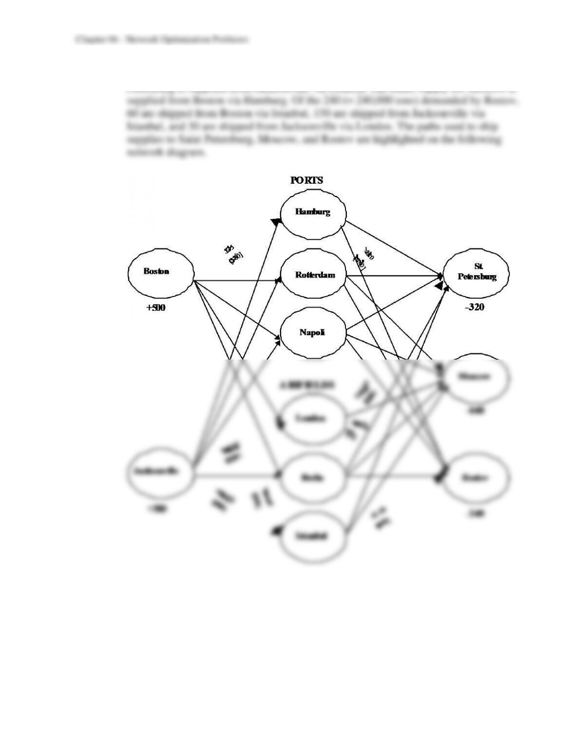
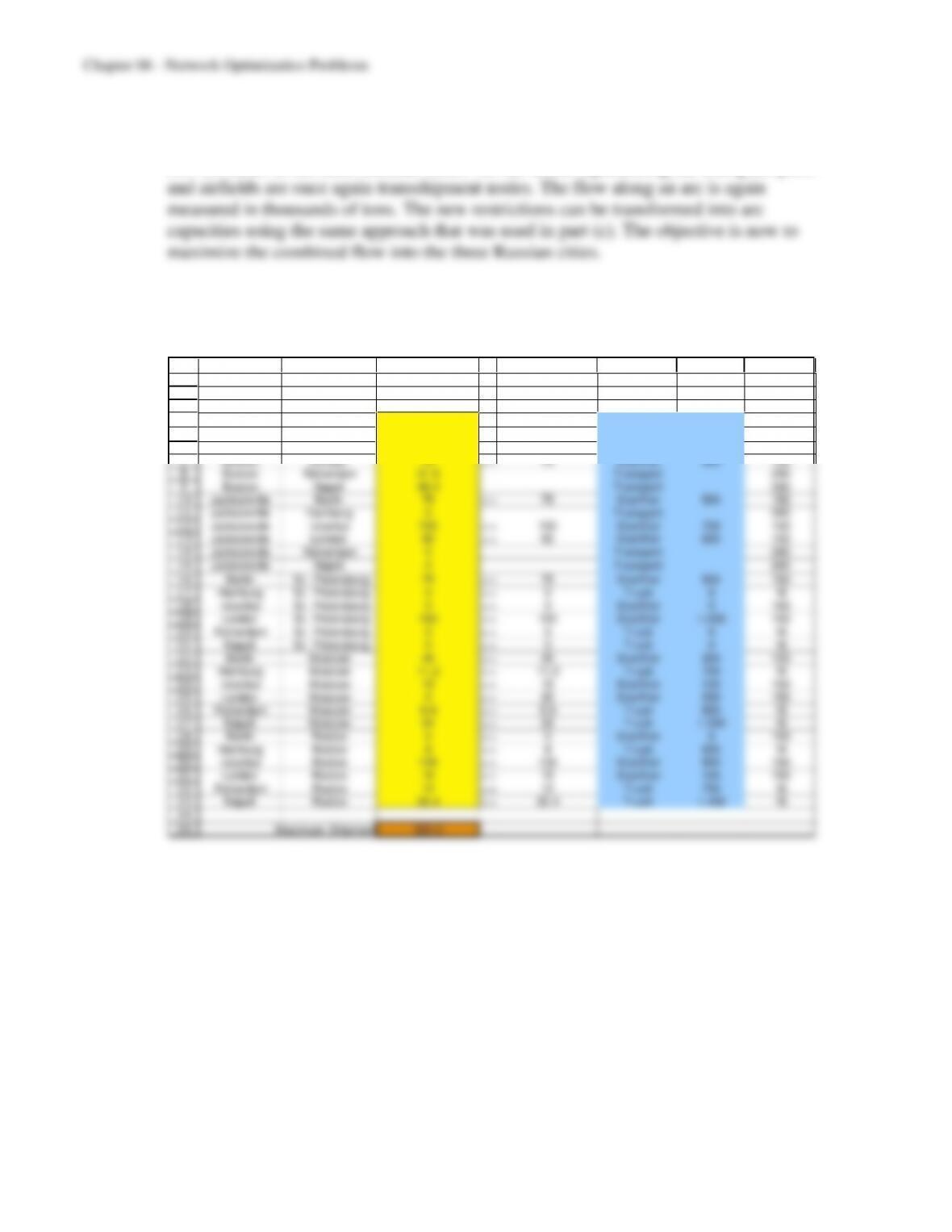
The total cost of the operation equals $412.867 million. The entire supply for Saint
Petersburg is supplied from Jacksonville via London. The entire supply for Moscow is
6-24
d) Now the President wants to maximize the amount of cargo transported from the US to
the Russian cities. In other words, the President wants to maximize the flow from the
two US cities to the three Russian cities. All the nodes representing the European ports
The linear programming spreadsheet model describing the maximum flow problem
appears as follows.
1
2
3
4
5
6
7
8
9
10
11
12
13
14
15
16
17
18
19
20
21
22
23
24
25
26
27
28
29
30
31
32
33
34
35
A B C D E F G H
Vehicle
Ship Capacity Maximu m Capacity
From To (thousand tons) (thousand tons) Vehicle Vehicles (to ns)
Boston Berlin 45 <= 45 Starlifter 300 150
Boston Hamburg 19.2 Transport 240
Boston Istanbul 45 <= 75 Starlifter 500 150
Boston London 75 <= 75 Starlifter 500 150
Boston Rotterdam 21.6 Transport 240
Boston Napoli 46.4 Transport 240
Jacksonville Berlin 75 <= 75 Starlifter 500 150
Jacksonville Hamburg 0 Transport 240
Jacksonville Istanbul 105 <= 105 Starlifter 700 150
Jacksonville London 90 <= 90 Starlifter 600 150
Jacksonville Rotterdam 0 Transport 240
Jacksonville Napoli 0 Transport 240
Berlin St. Petersburg 75 <= 75 Starlifter 500 150
Hamburg St. Petersburg 0 <= 0 Truck 0 16
Istanbul St. Petersburg 0 <= 0 Starlifter 0 150
London St. Petersburg 150 <= 150 Starlifter 1,000 150
Rotterdam St. Petersburg 0 <= 0 Truck 0 16
Napoli St. Petersburg 0 <= 0 Truck 0 16
Berlin Moscow 45 <= 45 Starlifter 300 150
Hamburg Moscow 11.2 <= 11.2 Truck 700 16
Istanbul Moscow 15 <= 15 Starlifter 100 150
London Moscow 0 <= 30 Starlifter 200 150
Rotterdam Moscow 9.6 <= 9.6 Truck 600 16
Napoli Moscow 24 <= 24 T ruck 1,500 16
Berlin Rostov 0 <= 0 Starlifter 0 150
Hamburg Rostov 8 <= 8 T ruck 500 16
Istanbul Rostov 135 <= 135 Starlifter 900 150
London Rostov 15 <= 15 Starlifter 100 150
Rotterdam Rostov 12 <= 12 Truck 750 16
Napoli Rostov 22.4 <= 22.4 T ruck 1,400 16
Maximum Shipment 522.2
6-25
1
2
3
4
5
6
7
8
9
10
11
12
13
14
15
16
17
18
19
20
21
22
J K L M
Net Flow Supp ly/Demand
Node (thousand tons) (thousand tons
Boston 252.2
Jacksonville 270
Berlin 0 = 0
Hamburg 0 = 0
Istanbul 0 = 0
London 0 = 0
Rotterdam 0 = 0
Napoli 0 = 0
St. Petersburg -225
Moscow -104.8
Rostov -192.4
Capacity
(tons)
Starlifter 150
Transport 240
Truck 16
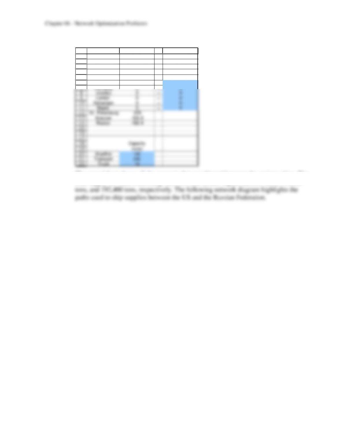
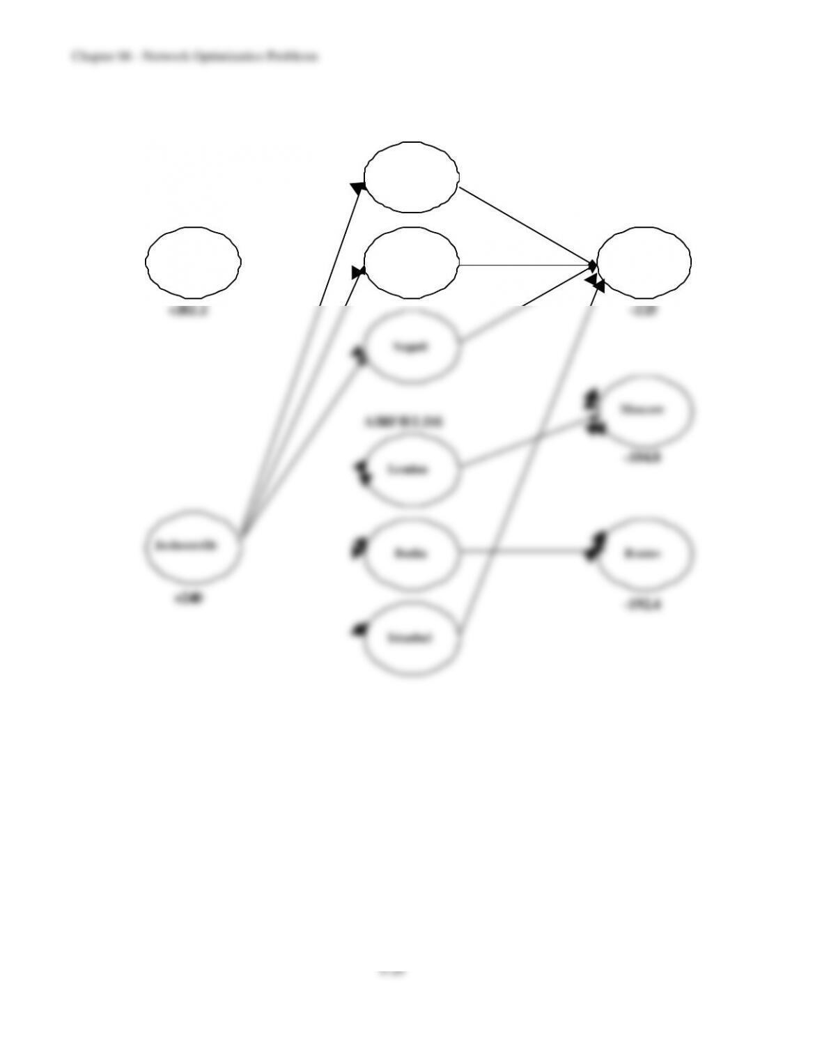
The spreadsheet shows all the amounts that are shipped between the various cities. The
total supply for Saint Petersburg, Moscow, and Rostov equals 225,000 tons, 104,800
6-27
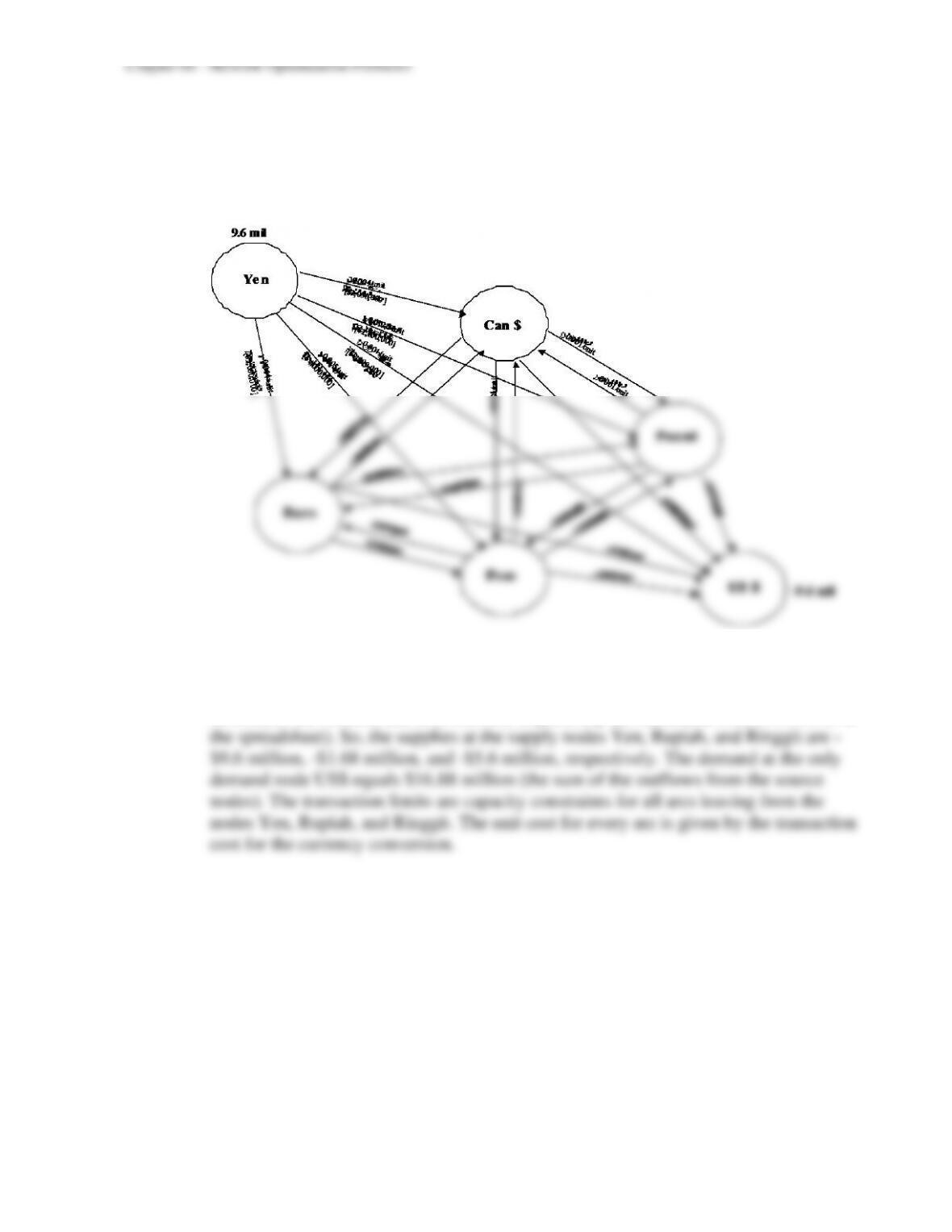
6.2 a) There are three supply nodes – the Yen node, the Rupiah node, and the Ringgit node.
There is one demand node – the US$ node. Below, we draw the network originating
from only the Yen supply node to illustrate the overall design of the network. In this
network, we exclude both the Rupiah and Ringgit nodes for simplicity.
b) Since all transaction limits are given in the equivalent of $1000 we define the flow
variables as the amount in thousands of dollars that Jake converts from one currency
into another one. His total holdings in Yen, Rupiah, and Ringgit are equivalent to $9.6
million, $1.68 million, and $5.6 million, respectively (as calculated in cells I16:K18 in
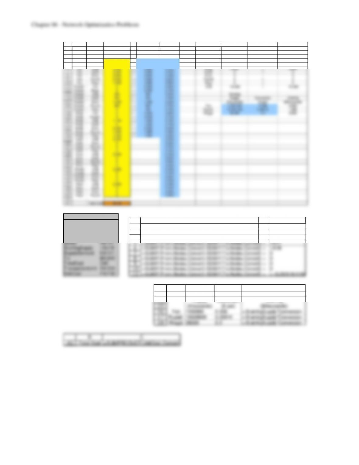
6-28
42
1
2
3
4
5
6
7
8
9
10
11
12
13
14
15
16
17
18
19
20
21
22
23
24
25
26
27
28
29
30
31
32
33
34
35
36
37
38
39
40
41
A B C D E F G H I J K
Transaction
Convert L imit Unit Net F low Su pply/Demand
From To ($th ousands) ($thousands) Cost Nodes ($thousands) ($thousands)
Yen Rupiah 0 <= 5,000 0.50% Yen 9,600 = 9,600
Yen Ringit 0 <= 5,000 0.50% Rupiah 1,680 = 1,680
Yen US$ 2,000 <= 2,000 0.40% Ringit 5,600 = 5,600
Yen Can$ 2,000 <= 2,000 0.40% Can$ 0 = 0
Yen Euro 2,000 <= 2,000 0.40% Euro 0 = 0
Yen Pound 2,000 <= 2,000 0.25% Pound 0 = 0
Yen Peso 1,600 <= 4,000 0.50% Peso 0 = 0
Rupiah Yen 0 <= 5,000 0.50% US$ –16,880 = -16,880
Rupiah Ringit 0 <= 2,000 0.70%
Rupiah US$ 200 <= 200 0.50% Starting
Rupiah Can$ 200 <= 200 0.30% Supply Conversion Starting
Rupiah Euro 1,000 <= 1,000 0.30% (thousands) ($ per) ($thousands)
Rupiah Pound 280 <= 500 0.75% Yen 1,200,000 0.008 9,600
Rupiah Peso 0 <= 200 0.75% Rupiah 10,500,000 0.00016 1,680
Ringit Yen 0 <= 3,000 0.50% Ringgit 28,000 0.2 5,600
Ringit Rupiah 0 <= 4,500 0.70%
Ringit US$ 1,100 <= 1,500 0.70%
Ringit Can$ 0 <= 1,500 0.70%
Ringit Euro 2,500 <= 2,500 0.40%
Ringit Pound 1,000 <= 1,000 0.45%
Ringit Peso 1,000 <= 1,000 0.50%
Can$ US$ 2,200 0.05%
Can$ Euro 0 0.20%
Can$ Pound 0 0.10%
Can$ Peso 0 0.10%
Euro US$ 5,500 0.10%
Euro Can$ 0 0.20%
Euro Pound 0 0.05%
Euro Peso 0 0.50%
Pound US$ 3,280 0.10%
Pound Can$ 0 0.10%
Pound Euro 0 0.05%
Pound Peso 0 0.50%
Peso US$ 2,600 0.10%
Peso Can$ 0 0.10%
Peso Euro 0 0.50%
Peso Pound 0 0.50%
Range Name Cells
Conversion J16:J18
Convert C4:C40
From A4:A40
NetFlow I4:I11
Nodes H4:H11
StartingSupply I16:I18
SupplyDemand K4:K11
To B4:B40
TotalCost C42
TransactionLimit E4:E24
UnitCost F4:F40
2
3
4
5
6
7
8
9
10
11
I J K
Net Flow Supply/Demand
($thousands) ($thousands)
=SUMIF(From,Nodes,Convert)-SUMIF(To,Nodes,Convert) = =K16
=SUMIF(From,Nodes,Convert)-SUMIF(To,Nodes,Convert) = =K17
=SUMIF(From,Nodes,Convert)-SUMIF(To,Nodes,Convert) = =K18
=SUMIF(From,Nodes,Convert)-SUMIF(To,Nodes,Convert) = 0
=SUMIF(From,Nodes,Convert)-SUMIF(To,Nodes,Convert) = 0
=SUMIF(From,Nodes,Convert)-SUMIF(To,Nodes,Convert) = 0
=SUMIF(From,Nodes,Convert)-SUMIF(To,Nodes,Convert) = 0
=SUMIF(From,Nodes,Convert)-SUMIF(To,Nodes,Convert) = =-SUM(K16:K18)
13
14
15
16
17
H I J K
Starting
Supply Conversion Starting
(thousands) ($ per) ($thousands)
Yen 1200000 0.008 = StartingSupply*Conversion
Rupiah 10500000 0.00016 = StartingSupply*Conversion
42
B C
Total Cost =SUMPRODUCT(UnitCost,Convert)
6-29
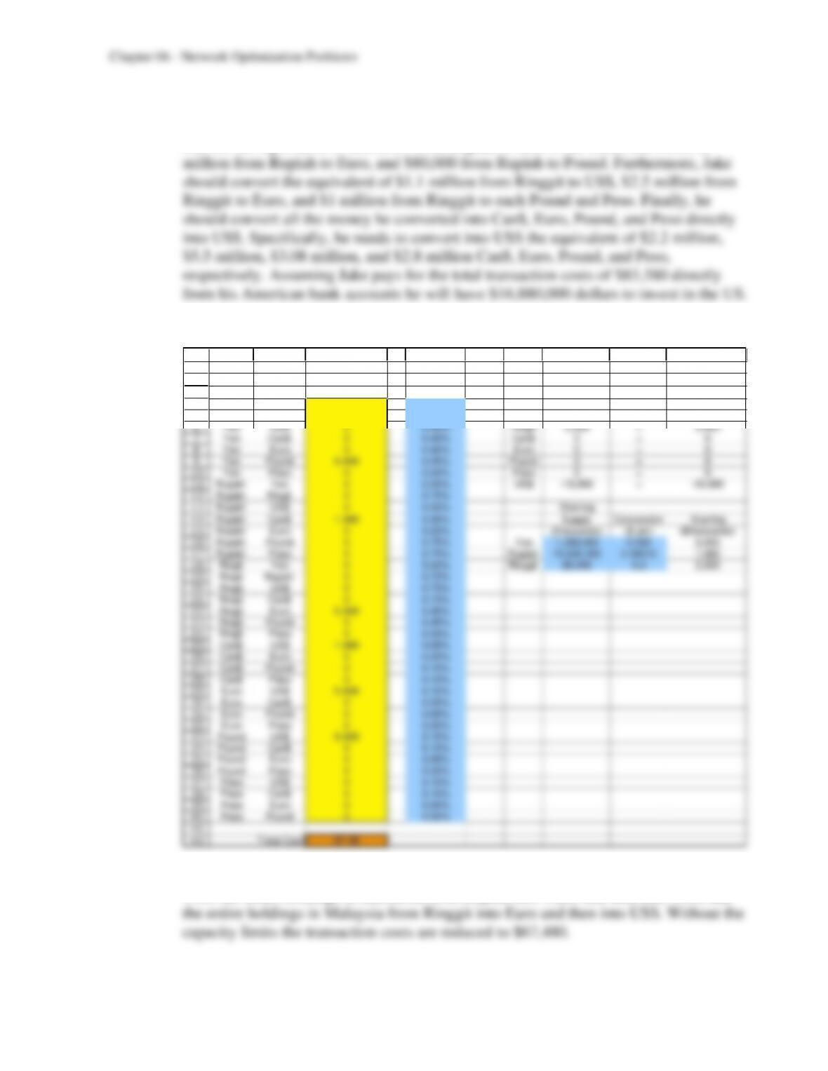
Jake should convert the equivalent of $2 million from Yen to each US$, Can$, Euro,
and Pound. He should convert $1.6 million from Yen to Peso. Moreover, he should
convert the equivalent of $200,000 from Rupiah to each US$, Can$, and Peso, $1
c) We eliminate all capacity restrictions on the arcs.
1
2
3
4
5
6
7
8
9
10
11
12
13
14
15
16
17
18
19
20
21
22
23
24
25
26
27
28
29
30
31
32
33
34
35
36
37
38
39
40
41
42
A B C D E F G H I J
Con vert Unit Net Flow Sup ply/Demand
From To ($th ousands) Cost Nodes ($th ousands) ($thou sands)
Yen Rupiah 0 0.50% Yen 9,600 = 9,600
Yen Ringit 0 0.50% Rupiah 1,680 = 1,680
Yen US$ 0 0.40% Ringit 5,600 = 5,600
Yen Can$ 0 0.40% Can$ 0 = 0
Yen Euro 0 0.40% Euro 0 = 0
Yen Pound 9,600 0.25% Pound 0 = 0
Yen Peso 0 0.50% Peso 0 = 0
Rupiah Yen 0 0.50% US$ –16,880 = -16,880
Rupiah Ringit 0 0.70%
Rupiah US$ 0 0.50% Starting
Rupiah Can$ 1,680 0.30% Supply Conversion Starting
Rupiah Euro 0 0.30% (thousands) ($ per) ($thousands)
Rupiah Pound 0 0.75% Yen 1,200,000 0.008 9,600
Rupiah Peso 0 0.75% Rupiah 10,500,000 0.00016 1,680
Ringit Yen 0 0.50% Ringgit 28,000 0.2 5,600
Ringit Rupiah 0 0.70%
Ringit US$ 0 0.70%
Ringit Can$ 0 0.70%
Ringit Euro 5,600 0.40%
Ringit Pound 0 0.45%
Ringit Peso 0 0.50%
Can$ US$ 1,680 0.05%
Can$ Euro 0 0.20%
Can$ Pound 0 0.10%
Can$ Peso 0 0.10%
Euro US$ 5,600 0.10%
Euro Can$ 0 0.20%
Euro Pound 0 0.05%
Euro Peso 0 0.50%
Pound US$ 9,600 0.10%
Pound Can$ 0 0.10%
Pound Euro 0 0.05%
Pound Peso 0 0.50%
Peso US$ 0 0.10%
Peso Can$ 0 0.10%
Peso Euro 0 0.50%
Peso Pound 0 0.50%
Total Cost 67.48
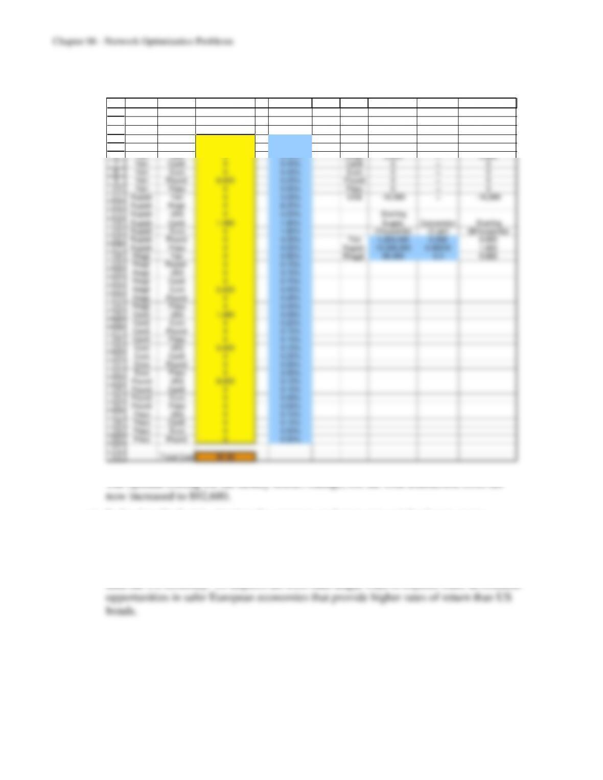
Jake should convert the entire holdings in Japan from Yen into Pounds and then into
US$, the entire holdings in Indonesia from Rupiah into Can$ and then into US$, and
6-30
d) We multiply all unit cost for Rupiah by 6.
1
2
3
4
5
6
7
8
9
10
11
12
13
14
15
16
17
18
19
20
21
22
23
24
25
26
27
28
29
30
31
32
33
34
35
36
37
38
39
40
41
42
A B C D E F G H I J
Con vert Unit Net Flow Sup ply/Demand
From To ($th ousands) Cost Nodes ($th ousands) ($thou sands)
Yen Rupiah 0 0.50% Yen 9,600 = 9,600
Yen Ringit 0 0.50% Rupiah 1,680 = 1,680
Yen US$ 0 0.40% Ringit 5,600 = 5,600
Yen Can$ 0 0.40% Can$ 0 = 0
Yen Euro 0 0.40% Euro 0 = 0
Yen Pound 9,600 0.25% Pound 0 = 0
Yen Peso 0 0.50% Peso 0 = 0
Rupiah Yen 0 3.00% US$ –16,880 = -16,880
Rupiah Ringit 0 4.20%
Rupiah US$ 0 3.00% Starting
Rupiah Can$ 1,680 1.80% Supply Conversion Starting
Rupiah Euro 0 1.80% (thousands) ($ per) ($thousands)
Rupiah Pound 0 4.50% Yen 1,200,000 0.008 9,600
Rupiah Peso 0 4.50% Rupiah 10,500,000 0.00016 1,680
Ringit Yen 0 0.50% Ringgit 28,000 0.2 5,600
Ringit Rupiah 0 0.70%
Ringit US$ 0 0.70%
Ringit Can$ 0 0.70%
Ringit Euro 5,600 0.40%
Ringit Pound 0 0.45%
Ringit Peso 0 0.50%
Can$ US$ 1,680 0.05%
Can$ Euro 0 0.20%
Can$ Pound 0 0.10%
Can$ Peso 0 0.10%
Euro US$ 5,600 0.10%
Euro Can$ 0 0.20%
Euro Pound 0 0.05%
Euro Peso 0 0.50%
Pound US$ 9,600 0.10%
Pound Can$ 0 0.10%
Pound Euro 0 0.05%
Pound Peso 0 0.50%
Peso US$ 0 0.10%
Peso Can$ 0 0.10%
Peso Euro 0 0.50%
Peso Pound 0 0.50%
Total Cost 92.68
The optimal routing for the money doesn’t change, but the total transaction costs are
e) In the described crisis situation the currency exchange rates might change every
minute. Jake should carefully check the exchange rates again when he performs the
transactions.
The European economies might be more insulated from the Asian financial collapse
than the US economy. To impress his boss Jake might want to explore other investment
6-31
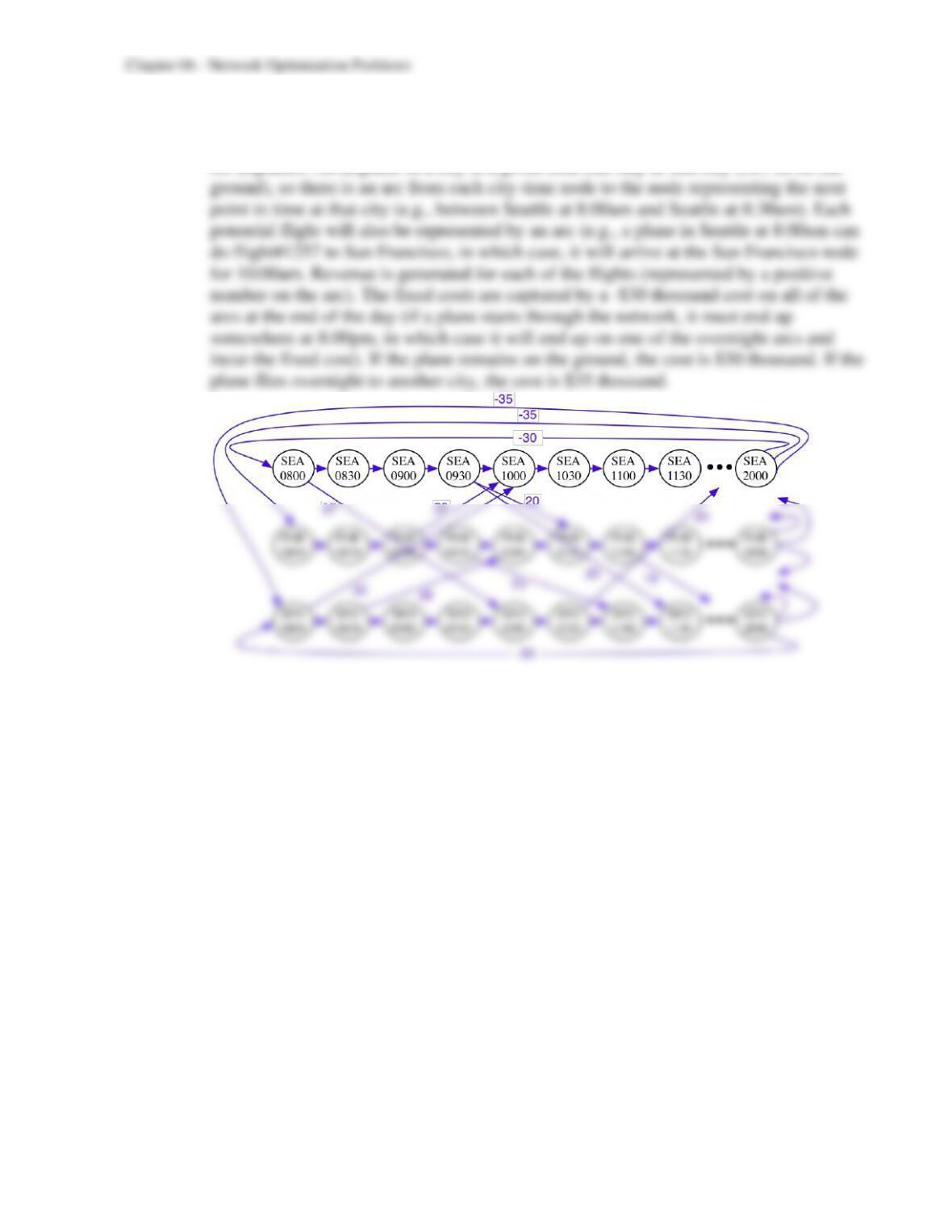
6.3 a) Each node represents a potential airplane location and point in time (e.g., Seattle at
8:00am, Seattle at 8:30am, Portland at 8:00am, etc.). The arcs represent potential paths
for airplanes. An airplane in a city at a given time can stay in that city (i.e., sit on the
6-32
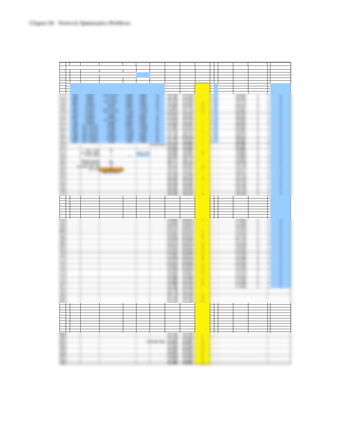
The spreadsheet solution for this problem is shown below. 16 flights are operated
generating a net profit of $307 thousand per day.
1
2
3
4
5
6
7
8
9
10
11
12
13
14
15
16
17
18
19
20
21
22
23
24
25
26
27
28
29
30
31
32
33
34
35
36
37
38
39
40
41
42
43
44
45
46
47
48
49
50
51
52
53
54
55
56
57
58
59
60
61
62
63
64
65
66
67
68
69
70
71
72
73
74
75
76
77
78
79
80
81
82
83
84
85
86
87
88
89
90
91
92
93
94
95
96
97
98
99
100
101
102
103
104
105
106
107
108
109
A B C D E F G H I J K L M N O P Q
Scheduling Flights at Northwest Commuter
Fixed Daily Cost of O perating Airplane 30 ($thousand)
Overnight Flight Cost 5 ($thousand)
Fligh t # From To Depart Arrive Revenue F rom To Flow Nodes Net Flow Supply/Demand
1257 Seattle San Francisco 8:00am 10:00am 37 SEA0800 SFO1000 1 <= 1 SEA0800 0 = 0
2576 Seattle Portland 9:30am 10:30am 20 SEA0930 POR1030 0 <= 1 SEA0830 0 = 0
8312 Seattle San Francisco 9:30am 11:30am 25 SEA0930 SF O1130 1 <= 1 SEA0900 0 = 0
1109 Seat t le San F rancisco 12:00pm 2:00pm 27 SEA1200 SFO 1400 1 <= 1 SEA0930 0 = 0
3752 Seattle San Francisco 2:30pm 4:30pm 23 SEA1430 SFO1630 1 <= 1 SEA1000 0 = 0
2498 Seattle Portland 3:00pm 4:00pm 18 SEA1500 POR1600 1 <= 1 SEA1030 0 = 0
8787 Seattle San Francisco 5:00pm 7:00pm 29 SEA1700 SFO1900 1 <= 1 SEA1100 0 = 0
8423 Seattle Portland 6:30pm 7:30pm 27 SEA1830 POR1930 0 <= 1 SEA1130 0 = 0
7922 Portland Seattle 9:00am 10:00am 20 POR0900 SEA1000 0 <= 1 SEA1200 0 = 0
5623 Portland San F rancisco 9:30am 11:00am 23 POR0930 SF O1100 0 <= 1 SEA1230 0 = 0
2448 Portland San F rancisco 11:00am 12:30pm 19 POR1100 SF O1230 0 <= 1 SEA1300 0 = 0
1842 Portland Seattle 12:00pm 1:00pm 21 PO R1200 SEA1300 1 <= 1 SEA1330 0 = 0
3487 Portland Seattle 2:00pm 3:00pm 22 POR1400 SEA1500 1 <= 1 SEA1400 0 = 0
4361 Portland San F rancisco 4:00pm 5:30pm 29 POR1600 SF O1730 1 <= 1 SEA1430 0 = 0
4299 Portland Seattle 6:00pm 7:00pm 27 POR1800 SEA1900 1 <= 1 SEA1500 0 = 0
1288 San Francisco Seattle 8:00am 10:00am 32 SFO 0800 SEA1000 1 <= 1 SEA1530 0 = 0
3335 San Francisco Portland 8:30am 10:00am 26 SF O 0830 PO R1000 1 <= 1 SEA1600 0 = 0
9348 San Francisco Seattle 10:30am 12:30pm 24 SF O 1030 SEA1230 0 <= 1 SEA1630 0 = 0
7400 San Francisco Seattle 12:00pm 2:00pm 27 SFO1200 SEA1400 1 <= 1 SEA1700 0 = 0
7328 San Francisco Portland 12:00pm 1:30pm 24 SFO 1200 POR1330 1 <= 1 SEA1730 0 = 0
6386 San Francisco Portland 4:00pm 5:30pm 28 SF O 1600 PO R1730 1 <= 1 SEA1800 0 = 0
6923 San Francisco Seattle 5:00pm 7:00pm 32 SFO1700 SEA1900 1 <= 1 SEA1830 0 = 0
Ground Arcs: SEA0800 SEA0830 1 SEA1900 0 = 0
SEA0830 SEA0900 1 SEA1930 0 = 0
Flights F lown 16 SEA0900 SEA0930 1 SEA2000 0 = 0
Overnight Flights 0 Planes O wned SEA0930 SEA1000 0 POR0800 0 = 0
Planes Used 4 <= 4 SEA1000 SEA1030 1 POR0830 0 = 0
SEA1030 SEA1100 1 PO R0900 0 = 0
Total Net Revenue 427 SEA1100 SEA1130 1 PO R0930 0 = 0
Total Fixed Cost 120 SEA1130 SEA1200 1 POR1000 0 = 0
Overnight Flight Cost 0 SEA1200 SEA1230 0 POR1030 0 = 0
Net Profit 307 SEA1230 SEA1300 0 POR1100 0 = 0
($thousand/ day) SEA1300 SEA1330 1 PO R1130 0 = 0
SEA1330 SEA1400 1 POR1200 0 = 0
SEA1400 SEA1430 2 POR1230 0 = 0
SEA1430 SEA1500 1 POR1300 0 = 0
SEA1500 SEA1530 1 POR1330 0 = 0
SEA1530 SEA1600 1 POR1400 0 = 0
SEA1600 SEA1630 1 POR1430 0 = 0
SEA1630 SEA1700 1 POR1500 0 = 0
SEA1700 SEA1730 0 POR1530 0 = 0
SEA1730 SEA1800 0 POR1600 0 = 0
SEA1800 SEA1830 0 POR1630 0 = 0
SEA1830 SEA1900 0 POR1700 0 = 0
SEA1900 SEA1930 2 POR1730 0 = 0
SEA1930 SEA2000 2 POR1800 0 = 0
PO R0800 PO R0830 0 POR1830 0 = 0
PO R0830 PO R0900 0 POR1900 0 = 0
PO R0900 PO R0930 0 POR1930 0 = 0
PO R0930 PO R1000 0 POR2000 0 = 0
PO R1000 PO R1030 1 SFO0800 0 = 0
PO R1030 PO R1100 1 SFO 0830 0 = 0
PO R1100 PO R1130 1 SFO 0900 0 = 0
PO R1130 PO R1200 1 SFO0930 0 = 0
PO R1200 PO R1230 0 SFO1000 0 = 0
PO R1230 PO R1300 0 SFO1030 0 = 0
PO R1300 PO R1330 0 SFO 1100 0 = 0
PO R1330 PO R1400 1 SFO 1130 0 = 0
PO R1400 PO R1430 0 SFO1200 0 = 0
PO R1430 PO R1500 0 SFO1230 0 = 0
PO R1500 PO R1530 0 SFO1300 0 = 0
PO R1530 PO R1600 0 SFO1330 0 = 0
PO R1600 PO R1630 0 SFO1400 0 = 0
PO R1630 PO R1700 0 SFO1430 0 = 0
PO R1700 PO R1730 0 SFO1500 0 = 0
PO R1730 PO R1800 1 SFO1530 0 = 0
PO R1800 PO R1830 0 SFO1600 0 = 0
PO R1830 PO R1900 0 SFO1630 0 = 0
PO R1900 PO R1930 0 SFO1700 0 = 0
PO R1930 PO R2000 0 SFO1730 0 = 0
SF O0800 SFO0830 1 SFO1800 0 = 0
SF O0830 SFO0900 0 SFO1830 0 = 0
SF O0900 SFO0930 0 SFO1900 0 = 0
SF O0930 SFO1000 0 SFO1930 0 = 0
SF O1000 SFO1030 1 SFO2000 0 = 0
SF O1030 SFO1100 1
SF O1100 SFO1130 1
SF O1130 SFO1200 2
SF O1200 SFO1230 0
SF O1230 SFO1300 0
SF O1300 SFO1330 0
SF O1330 SFO1400 0
SF O1400 SFO1430 1
SF O1430 SFO1500 1
SF O1500 SFO1530 1
SF O1530 SFO1600 1
SF O1600 SFO1630 0
SF O1630 SFO1700 1
SF O1700 SFO1730 0
SF O1730 SFO1800 1
SF O1800 SFO1830 1
SF O1830 SFO1900 1
SF O1900 SFO1930 2
SF O1930 SFO2000 2
Overnig h t Arcs: SEA2000 SEA0800 2
PO R2000 PO R0800 0
SF O2000 SFO0800 2
SEA2000 POR0800 0
SEA2000 SFO 0800 0
PO R2000 SEA0800 0
PO R2000 SF O 0800 0
SF O2000 SEA0800 0
SF O2000 POR0800 0
6-33
b) A Data Table was generated, to show the NetProfit (D38) as the number in
PlanesOwned (F33) is varied between 4 and 7. The results are shown below. The fifth
43
44
45
46
47
48
C D
Planes O wned Net Profit
355
4 307
5 351
6 355
7 355
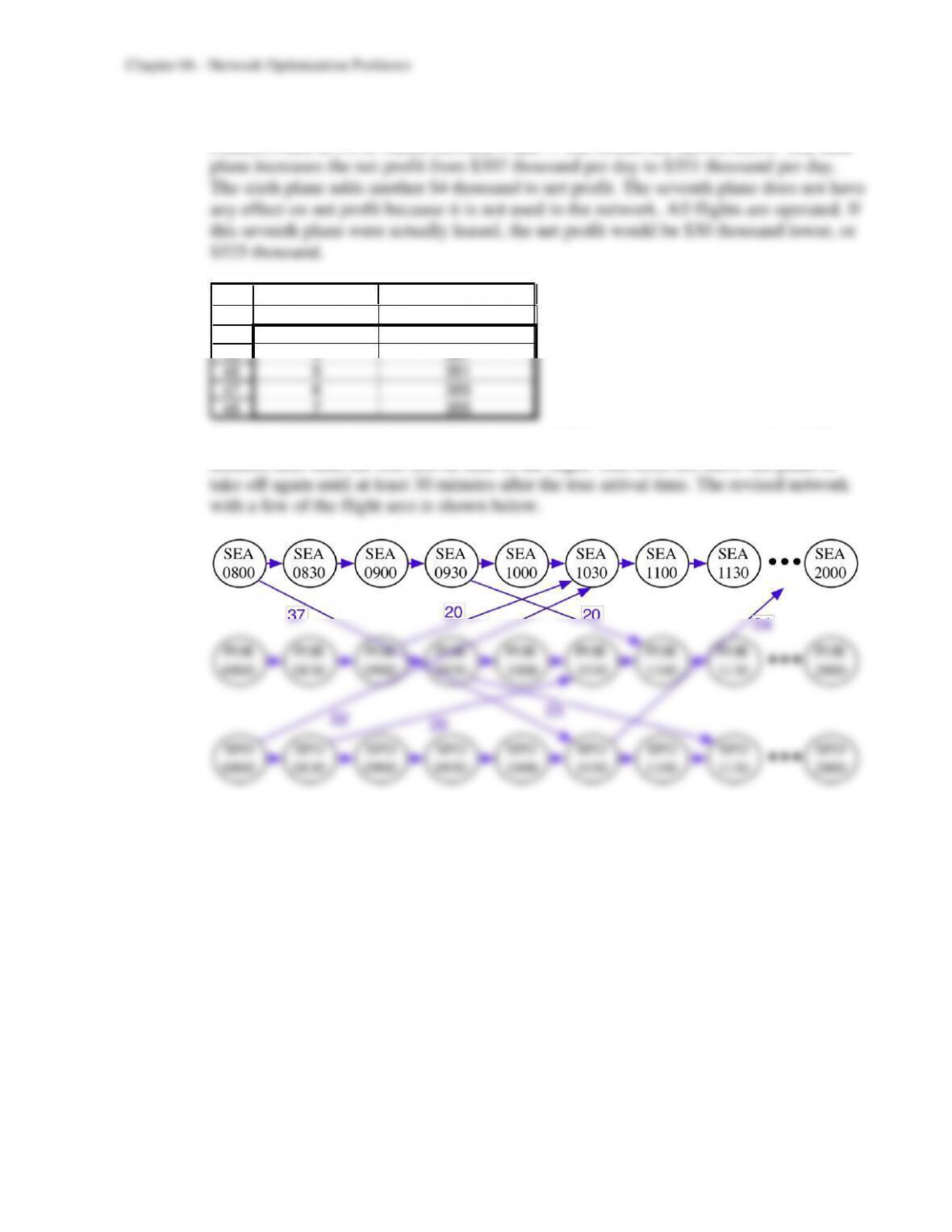
c) The network from part a is modified so that all flight arcs end at the node that is 30
minutes later than the true arrival time of the flight. This does not allow the plane to
6-34
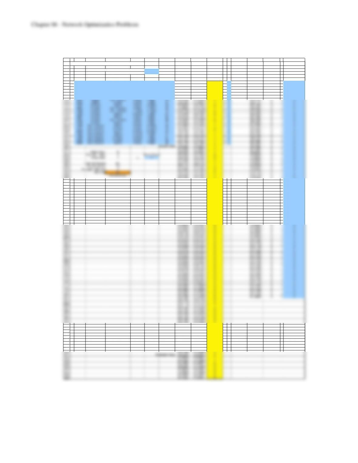
The spreadsheet solution for the revised network is shown below. The new solution
operates 15 flights and generates a net revenue of $287 thousand per day.
1
2
3
4
5
6
7
8
9
10
11
12
13
14
15
16
17
18
19
20
21
22
23
24
25
26
27
28
29
30
31
32
33
34
35
36
37
38
39
40
41
42
43
44
45
46
47
48
49
50
51
52
53
54
55
56
57
58
59
60
61
62
63
64
65
66
67
68
69
70
71
72
73
74
75
76
77
78
79
80
81
82
83
84
85
86
87
88
89
90
91
92
93
94
95
96
97
98
99
100
101
102
103
104
105
106
107
108
109
A B C D E F G H I J K L M N O P Q
Scheduling Flights at Northwest Commuter
Fixed Daily Cost of O perating Airplane 30 ($thousand)
Overnight Flight Cost 5 ($thousand)
Fligh t # From To Depart Arrive Revenue F rom To F low Nodes Net F low Su pply/Demand
1257 Seattle San Francisco 8:00am 10:00am 37 SEA0800 SFO 1030 1 <= 1 SEA0800 0 = 0
2576 Seattle Portland 9:30am 10:30am 20 SEA0930 PO R1100 0 <= 1 SEA0830 0 = 0
8312 Seattle San Francisco 9:30am 11:30am 25 SEA0930 SFO 1200 1 <= 1 SEA0900 0 = 0
1109 Seat tle San F rancisco 12:00pm 2:00pm 27 SEA1200 SFO1430 1 <= 1 SEA0930 0 = 0
3752 Seattle San Francisco 2:30pm 4:30pm 23 SEA1430 SFO 1700 1 <= 1 SEA1000 0 = 0
2498 Seattle Portland 3:00pm 4:00pm 18 SEA1500 PO R1630 0 <= 1 SEA1030 0 = 0
8787 Seattle San Francisco 5:00pm 7:00pm 29 SEA1700 SFO 1930 1 <= 1 SEA1100 0 = 0
8423 Seattle Portland 6:30pm 7:30pm 27 SEA1830 PO R2000 1 <= 1 SEA1130 0 = 0
7922 Portland Seattle 9:00am 10:00am 20 POR0900 SEA1030 0 <= 1 SEA1200 0 = 0
5623 Portland San F rancisco 9:30am 11:00am 23 POR0930 SFO 1130 1 <= 1 SEA1230 0 = 0
2448 Portland San F rancisco 11:00am 12:30pm 19 POR1100 SF O1300 0 <= 1 SEA1300 0 = 0
1842 Portland Seattle 12:00pm 1:00pm 21 POR1200 SEA1330 0 <= 1 SEA1330 0 = 0
3487 Portland Seattle 2:00pm 3:00pm 22 POR1400 SEA1530 1 <= 1 SEA1400 0 = 0
4361 Portland San F rancisco 4:00pm 5:30pm 29 POR1600 SFO1800 0 <= 1 SEA1430 0 = 0
4299 Portland Seattle 6:00pm 7:00pm 27 POR1800 SEA1930 1 <= 1 SEA1500 0 = 0
1288 San Francisco Seattle 8:00am 10:00am 32 SFO 0800 SEA1030 1 <= 1 SEA1530 0 = 0
3335 San Francisco Portland 8:30am 10:00am 26 SF O0830 POR1030 0 <= 1 SEA1600 0 = 0
9348 San Francisco Seattle 10:30am 12:30pm 24 SF O1030 SEA1300 1 <= 1 SEA1630 0 = 0
7400 San Francisco Seattle 12:00pm 2:00pm 27 SFO1200 SEA1430 1 <= 1 SEA1700 0 = 0
7328 San Francisco Portland 12:00pm 1:30pm 24 SFO 1200 PO R1400 1 <= 1 SEA1730 0 = 0
6386 San Francisco Portland 4:00pm 5:30pm 28 SF O 1600 PO R1800 1 <= 1 SEA1800 0 = 0
6923 San Francisco Seattle 5:00pm 7:00pm 32 SFO1700 SEA1930 1 <= 1 SEA1830 0 = 0
Groun d Arcs: SEA0800 SEA0830 1 SEA1900 0 = 0
SEA0830 SEA0900 1 SEA1930 0 = 0
Flights F lown 15 SEA0900 SEA0930 1 SEA2000 0 = 0
Overnight Flights 0 Planes O wned SEA0930 SEA1000 0 PO R0800 0 = 0
Planes Used 4 <= 4 SEA1000 SEA1030 0 POR0830 0 = 0
SEA1030 SEA1100 1 POR0900 0 = 0
Total Net Revenue 407 SEA1100 SEA1130 1 POR0930 0 = 0
Total Fixed Cost 120 SEA1130 SEA1200 1 PO R1000 0 = 0
Overnight Flight Cost 0 SEA1200 SEA1230 0 PO R1030 0 = 0
Net Profit 287 SEA1230 SEA1300 0 POR1100 0 = 0
($thousand/day) SEA1300 SEA1330 1 POR1130 0 = 0
SEA1330 SEA1400 1 PO R1200 0 = 0
SEA1400 SEA1430 1 PO R1230 0 = 0
SEA1430 SEA1500 1 PO R1300 0 = 0
SEA1500 SEA1530 1 PO R1330 0 = 0
SEA1530 SEA1600 2 PO R1400 0 = 0
SEA1600 SEA1630 2 PO R1430 0 = 0
SEA1630 SEA1700 2 PO R1500 0 = 0
SEA1700 SEA1730 1 PO R1530 0 = 0
SEA1730 SEA1800 1 PO R1600 0 = 0
SEA1800 SEA1830 1 PO R1630 0 = 0
SEA1830 SEA1900 0 PO R1700 0 = 0
SEA1900 SEA1930 0 PO R1730 0 = 0
SEA1930 SEA2000 2 PO R1800 0 = 0
PO R0800 PO R0830 1 PO R1830 0 = 0
PO R0830 PO R0900 1 PO R1900 0 = 0
PO R0900 PO R0930 1 PO R1930 0 = 0
PO R0930 PO R1000 0 PO R2000 0 = 0
PO R1000 PO R1030 0 SF O0800 0 = 0
PO R1030 PO R1100 0 SFO0830 0 = 0
PO R1100 PO R1130 0 SFO0900 0 = 0
PO R1130 PO R1200 0 SF O0930 0 = 0
PO R1200 PO R1230 0 SF O1000 0 = 0
PO R1230 PO R1300 0 SF O1030 0 = 0
PO R1300 PO R1330 0 SFO1100 0 = 0
PO R1330 PO R1400 0 SFO1130 0 = 0
PO R1400 PO R1430 0 SF O1200 0 = 0
PO R1430 PO R1500 0 SF O1230 0 = 0
PO R1500 PO R1530 0 SF O1300 0 = 0
PO R1530 PO R1600 0 SF O1330 0 = 0
PO R1600 PO R1630 0 SF O1400 0 = 0
PO R1630 PO R1700 0 SF O1430 0 = 0
PO R1700 PO R1730 0 SF O1500 0 = 0
PO R1730 PO R1800 0 SF O1530 0 = 0
PO R1800 PO R1830 0 SF O1600 0 = 0
PO R1830 PO R1900 0 SF O1630 0 = 0
PO R1900 PO R1930 0 SF O1700 0 = 0
PO R1930 PO R2000 0 SF O1730 0 = 0
SF O0800 SFO 0830 0 SF O1800 0 = 0
SF O0830 SFO 0900 0 SF O1830 0 = 0
SF O0900 SFO 0930 0 SF O1900 0 = 0
SF O0930 SFO 1000 0 SF O1930 0 = 0
SF O1000 SFO 1030 0 SF O2000 0 = 0
SF O1030 SFO 1100 0
SF O1100 SFO 1130 0
SF O1130 SFO 1200 1
SF O1200 SFO 1230 0
SF O1230 SFO 1300 0
SF O1300 SFO 1330 0
SF O1330 SFO 1400 0
SF O1400 SFO 1430 0
SF O1430 SFO 1500 1
SF O1500 SFO 1530 1
SF O1530 SFO 1600 1
SF O1600 SFO 1630 0
SF O1630 SFO 1700 0
SF O1700 SFO 1730 0
SF O1730 SFO 1800 0
SF O1800 SFO 1830 0
SF O1830 SFO 1900 0
SF O1900 SFO 1930 0
SF O1930 SFO 2000 1
Overnig ht Arcs: SEA2000 SEA0800 2
PO R2000 PO R0800 1
SF O2000 SFO 0800 1
SEA2000 POR0800 0
SEA2000 SFO 0800 0
PO R2000 SEA0800 0
PO R2000 SF O0800 0
SF O2000 SEA0800 0
SF O2000 POR0800 0
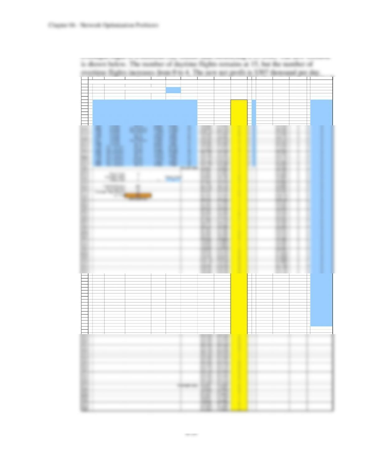
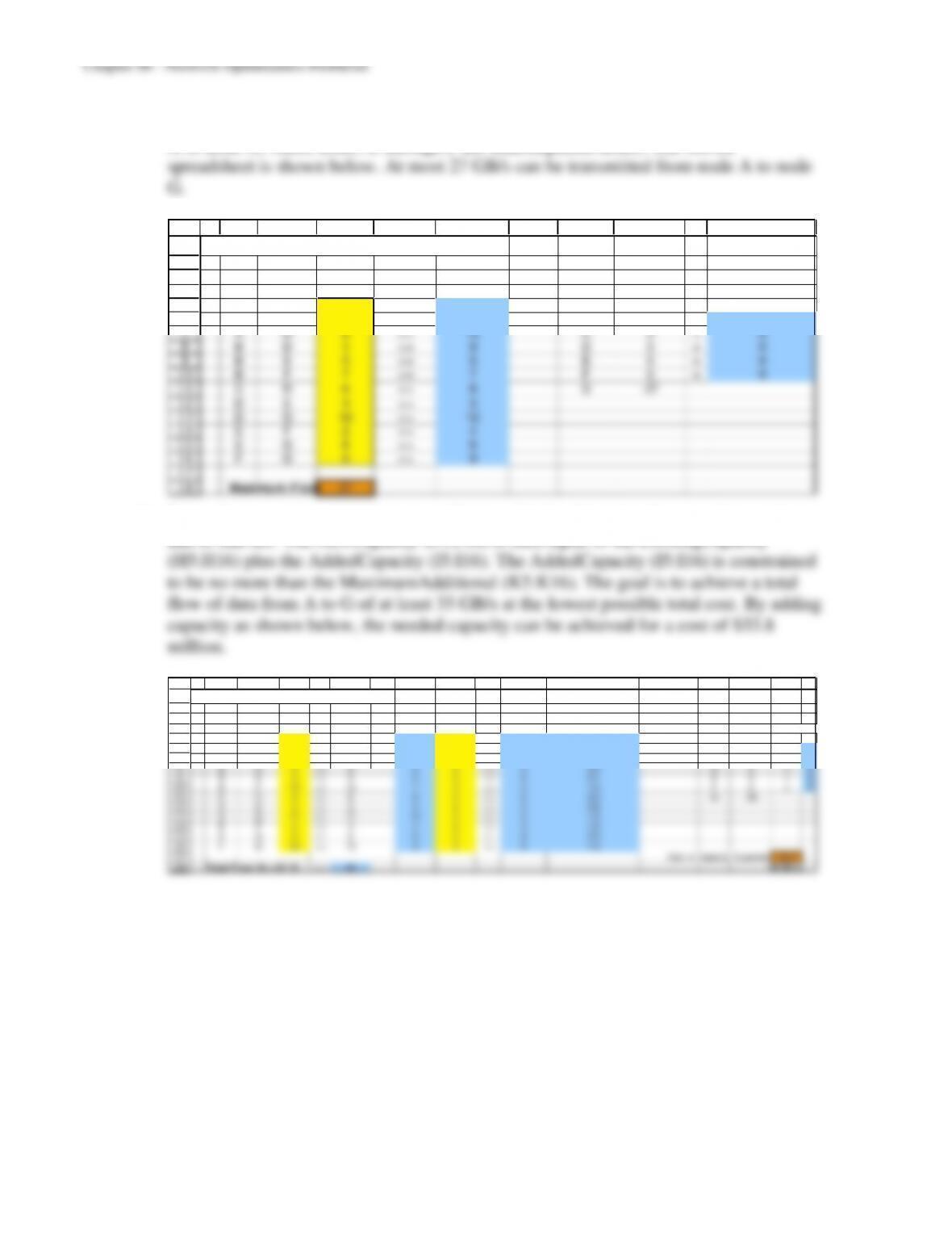
6-36
6.4 a) This is a maximum flow problem. The goal is to maximize the flow of data from node
A to node G, where nodes B through F are transshipment nodes. The solved
1
2
3
4
5
6
7
8
9
10
11
12
13
14
15
16
17
18
A B C D E F G H I J K
Broadcasting the Olympic Games
Existing
Flow Cap acity Net F low
From To (GB/s) (G B/s) Nodes (GB/s) Supp ly/Demand
A B 13 <= 13 A27
A C 6 <= 6 B 0 = 0
A D 8 <= 10 C 0 = 0
B D 1 <= 9 D 0 = 0
B E 5 <= 5 E 0 = 0
B F 7 <= 7 F 0 = 0
C D 6 <= 8 G -27
D E 3 <= 3
D G 12 <= 12
E F 2 <= 4
E G 6 <= 6
F G 9 <= 9
Maximum F low 27
b) For each arc, a new set of changing cells are added to determine how much capacity to
add to that arc. The NewCapacity (F5:F16) is then equal to the ExistingCapacity
1
2
3
4
5
6
7
8
9
10
11
12
13
14
15
16
17
18
A B C D E F G H I J K L M N O P Q
Broadcasting the Olympic Games
New Existing Added Maximum Cost per Gb ps
Flow Capacity Capacity Capacity Add itionalo f Add ition al Capacity Net F low
From To (G B/s) (GB/s) (GB/s) (GB/s) (GB/s) ($millions) Nodes (GB/s) Supp ly/D
A B 17 <= 17 13 4<= 6 2.8 A 35
A C 8 <= 8 6 2 <= 4 2.5 B 0 = 0
A D 10 <= 10 10 0<= 3 2.8 C 0 = 0
B D 2 <= 9 9 0 <= 4 2.5 D 0 = 0
B E 5 <= 5 5 0 <= 5 3.1 E 0 = 0
B F 10 <= 10 7 3 <= 3 1.6 F 0 = 0
C D 8 <= 8 8 0 <= 5 3.9 G -35
D E 3 <= 3 3 0 <= 2 2.8
D G 17 <= 17 12 5<= 5 1.6
E F 2 <= 4 4 0 <= 2 4.6
E G 6 <= 6 6 0 <= 4 2.9
F G 12 <= 12 9 3 <= 5 1.6
Cost of Capacity Expansion 33.8
Total Flo w (A–> G) 35 >= 35 ($millions)