6-2
6-3
2. Whereas the number of supply nodes and the number of demand nodes in a minimum
6.3-5 Applications of maximum flow problems include maximizing the flow through a
6.4-1 The origin is the fire station and the destination is the farm community.
6.4-2 Flow can go in either direction between the nodes connected by links as opposed to only
one direction with an arc.
6.4-4 The length of a link can measure distance, cost, or time.
6.4-6 When “real travel” through a network can end at more that one node, a dummy destination
needs to be added so that the network will have just a single destination.
Problems
6.1 In this study, flight delay and cancellation problems faced by United Airlines (UA) are
modeled as minimum-cost-flow network models. The overall objective is to minimize a
weighted sum of various measures related to delay. These include the total number of delay
The delay problem is solved for each airport separately as a minimum-cost-flow network
problem. The flow on each arc can be at most one. The solution is a set of arcs starting at a
supply node and ending at a demand node, which determines flight delays due to shortage
6-4
This study has saved UA over half a billion dollars in delay costs alone in less than a year.
Many potential delays were prevented and hence the number of flight delays was reduced
6-6
6.4 a)
W1
W2
F1
F2
V1
V3
supply node s transshipme nt nodes de mand node
V2
b)
c)
1
2
3
4
5
6
7
8
9
10
11
12
13
14
15
16
17
18
19
20
21
22
23
24
A B C D E F G H I J K
Fixed Per Total Total
Shipping Mile Miles to Miles to Cost to Cost to
Vendor Price Charge Charge WH1 WH2 WH1 W H2
1 $22,500 $300 $0.40 1600 400 $23,440 $22,960
2 $22,700 $200 $0.50 500 600 $23,150 $23,200
3 $22,300 $500 $0.20 2000 1000 $23,200 $23,000
From To Ship Capacity Unit Cost Nodes Net Flow Supp ly/Demand
V1 WH1 0 <= 6 $23,440 V1 10 =10
V1 WH2 6 <= 6 $22,960 V2 10 =10
V2 WH1 6 <= 6 $23,150 V3 10 =10
V2 WH2 0 <= 6 $23,200 WH1 0 = 0
V3 WH1 0 <= 6 $23,200 WH2 0 = 0
V3 WH2 4 <= 6 $23,000 F1 –10 = -10
WH1 F1 6<= 6 $200 F2 -6 =-6
WH1 F2 0<= 6 $700 D –14 = -14
WH2 F1 4<= 6 $400
WH2 F2 6<= 6 $500
V1 D 4 $0
V2 D 4 $0
V3 D 6 $0
Total Cost $374,460
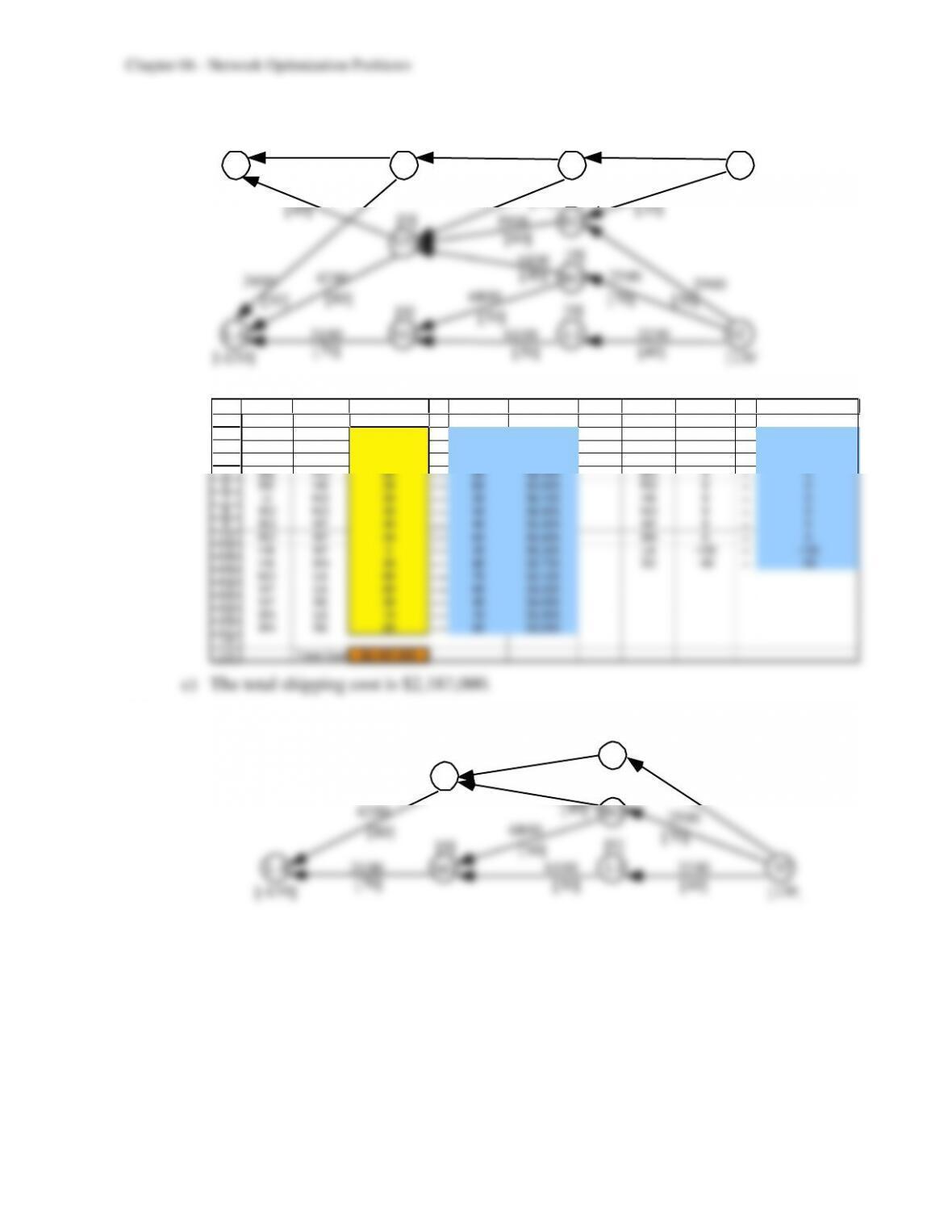
6.5 a)
BN
NO
HA
RO
BO
[0]
[0]
[50]
[130]
[–50]
[–130]
[20]
4000
[40]
4200
[80]
5700
[40] 6300
[30]
5900
5400
[60]
3100
[40]
6800
SE
LA
[10]
3400
NY
LI
BE
ST
[70]
[0]
[50]
6100
[30]
[0]
[0]
[0]
[0]
2000
[60]
2400
[20]
2900
[50]
2500
[70]
3200
[40]
3000
b)
1
2
3
4
5
6
7
8
9
10
11
12
13
14
15
16
17
18
19
A B C D E F G H I J K
From To Ship Capacity Unit Cost Nod es Net Flo w Supply/Demand
ST LI 30 <= 40 $3,200 ST 130 = 130
ST BO 70 <= 70 $2,500 BE 50 =50
ST RO 30 <= 50 $2,900 LI 0 = 0
BE RO 20 <= 20 $2,400 BO 0 = 0
BE HA 30 <= 60 $2,000 RO 0 = 0
LI NO 30 <= 30 $6,100 HA 0 = 0
BO NO 30 <= 50 $6,800 NO 0 = 0
BO NY 40 <= 40 $5,400 NY 0 = 0
RO NY 50 <= 60 $5,900 BN 0 = 0
HA NY 0<= 30 $6,300 LA -130 = -130
HA BN 30 <= 40 $5,700 SE -50 = –50
NO LA 60 <= 70 $3,100
NY LA 60 <= 80 $4,200
NY SE 30 <= 40 $4,000
BN LA 10 <= 10 $3,400
BN SE 20 <= 20 $3,000
Total Cost $2,187,000
c) The total shipping cost is $2,187,000.
6.6 a)
NO
RO
BO
[0]
[130]
[–130]
4200
[80]
5900
5400
[60]
3100
[40]
6800
LA
NY
LI ST
[70]
[0]
[50]
6100
[30]
[0]
[0]
[0]
2900
[50]
2500
[70]
3200
[40]
6.10 a)
A
C
D
E
[75]
[65]
[50]
[60]
[45]
[55]
[70]
R1
R3
[40]
B
F
T
[60] [45]
[70]
[120]
[190]
[130]
Sources
R2
[80]
[70] [90]
Transshipm ent Node s Si nk
b)
1
2
3
4
5
6
7
8
9
10
11
12
13
14
15
16
17
18
19
20
A B C D E F G H I J
From To Ship Capacity Nodes Net Flow Su pp ly/Deman d
R1 A65 <= 75 R1 95
R1 B30 <= 65 R2 150
R2 A40 <= 40 R3 150
R2 B50 <= 50 A 0 = 0
R2 C60 <= 60 B 0 = 0
R3 B80 <= 80 C 0 = 0
R3 C70 <= 70 D 0 = 0
A D 60 <= 60 E 0 = 0
A E 45 <= 45 F 0 = 0
B D 60 <= 70 T –395
B E 55 <= 55
B F 45 <= 45
C E 45 <= 70
C F 85 <= 90
D T 120 <= 120
E T 145 <= 190
F T 130 <= 130
Maximum Flow 395
6.11 a)
AK
SE
SF
TX
KC SL
NO
AT CH
PT
ME
CA
SF
b)
CA
TX
AK
ME SL
SE
CH
NO
SF
KC
AT
PT
Oil Fi el ds Refi nerie s Di st ri bu ti on
Cente rs
6-12
d)
1
2
3
4
5
6
7
8
9
10
11
12
13
14
15
16
17
18
19
20
21
22
23
24
25
26
27
28
29
30
31
32
33
34
35
A B C D E F G H I J
From To Ship Capacity Nodes Net Flo w Sup ply/Demand
Texas New Orleans 11 <= 11 T exas 28
Texas Charleston 7 <= 7 California 24
Texas Seattle 2 <= 2 Alaska 28
Texas St. Louis 8 <= 8 Middle East 28
California New O rleans 5 <= 5 New O rleans 0 = 0
California Charleston 4 <= 4 Charleston 0 = 0
California Seattle 8 <= 8 Seattle 0 = 0
California St. Louis 7 <= 7 St. Louis 0 = 0
Alaska New Orleans 7 <= 7 Pittsburgh -26
Alaska Charleston 3 <= 3 Atlanta –33
Alaska Seattle 12 <= 12 Kansas City –25
Alaska St. Louis 6 <= 6 San F rancisco –24
Middle East New O rleans 1 <= 8
Middle East Charleston 9 <= 9
Middle East Seattle 3 <= 4
Middle East St. Louis 15 <= 15
New O rleans Pittsburgh 5 <= 5
New O rleans Atlanta 9 <= 9
New O rleans Kansas City 6 <= 6
New O rleans San Francisco 4 <= 4
Charleston Pittsburgh 8 <= 8
Charleston Atlanta 7 <= 7
Charleston Kansas City 3 <= 9
Charleston San Francisco 5 <= 5
Seattle Pittsburgh 4 <= 4
Seattle Atlanta 6 <= 6
Seattle Kansas City 7 <= 7
Seattle San Francisco 8 <= 8
St. Louis Pittsburgh 9 <= 12
St. Louis Atlanta 11 <= 11
St. Louis Kansas City 9 <= 9
St. Louis San Francisco 7 <= 7
Maximum Flow 108
6.12 Prior to this study, Canadian Pacific Railway (CPR) used to run trains only after a
sufficient level of freight was attained. This policy resulted in unreliable delivery times, so
Developing the blocking plan, i.e., determining the group of railcars to move together at
some point during their trips, involves solving a series of shortest-path problems over a
6-13
This study enabled CPR to save $170 million in half a year. “Total documented cost
savings through the end of 2002 have exceeded half a billion dollars” [p. 12]. More savings
are expected in following years. The improvements in CPR’s profitability and operations
6.13
3
4
5
6
7
8
9
10
11
12
13
14
15
16
17
18
19
20
21
22
23
24
25
26
27
28
29
B C D E F G H I J K
From To O n Rou te Distance Nodes Net Flow Supply/Deman d
Fire St. A 0 3 Fire St. 1 = 1
Fire St. B 0 6 A 0 = 0
Fire St. C 1 4 B 0 = 0
A B 0 4 C 0 = 0
A D 0 6 D 0 = 0
B A 0 1 E 0 = 0
B C 0 2 F 0 = 0
B D 0 4 G 0 = 0
B E 0 5 H 0 = 0
C B 0 2 Farm Com. -1 =-1
C E 1 7
D E 0 3
D F 0 8
E D 0 3
E F 1 6
E G 0 5
E H 0 4
F G 0 3
F Farm Com. 1 4
G F 0 3
G H 0 2
G Farm Com. 0 6
H G 0 2
H Farm Com. 0 7
To tal Distance 21
Shortest path: Fire Station – C – E – F – Farming Community
6.14 a)
D
E
70
55
50
60
80
A
C
B40 10
OT
40
60
50
10
20
6-14
b)
1
2
3
4
5
6
7
8
9
10
11
12
13
14
15
16
17
18
19
20
21
A B C D E F G H I J
From To O n Route Distance (miles) Nod es Net Flow Supply/Deman d
Origin A 1 40 Origin 1 = 1
Origin B 0 60 A 0 = 0
Origin C 0 50 B 0 = 0
A B 1 10 C 0 = 0
A D 0 70 D 0 = 0
B A 0 10 E 0 = 0
B C 0 20 Destination -1 =-1
B D 0 55
B E 1 40
C B 0 20
C N 0 20
C E 0 50
D A 0 70
D B 0 55
D E 0 10
D Destination 1 60
E D 1 10
E Destination 0 80
Total Distance (miles) 160
c) Shortest route: Origin – A – B – E – D – Destination
d) Yes
e) Yes
6.15 a)
0 1 2 3
8, 000 10,000 12,000
18,000
31,000
21,000
b)
1
2
3
4
5
6
7
8
9
A B C D E F G H I J
From To On Route Cost Nodes Net F low Supply/Demand
Year 0 Year 1 1 $8,000 Year 0 1 = 1
Year 0 Year 2 0 $18,000 Year 1 0 = 0
Year 0 Year 3 0 $31,000 Year 2 0 = 0
Year 1 Year 2 0 $10,000 Year 3 -1 =-1
Year 1 Year 3 1 $21,000
Year 2 Year 3 0 $12,000
Total Cost $29,000
6.16 a) Times play the role of distances.
6-15
b)
1
2
3
4
5
6
7
8
9
10
11
12
13
14
15
16
A B C D E F G H I J
From To On Route Time (hours) Nodes Net Flow Su pply/Demand
Seattle A 0 4.6 Seattle 1 = 1
Seattle B 0 4.7 A 0 = 0
Seattle C 1 4.2 B 0 = 0
A D 0 3.5 C 0 = 0
A E 0 3.4 D 0 = 0
B D 0 3.6 E 0 = 0
B E 0 3.2 F 0 = 0
B F 0 3.3 London -1 =-1
C E 1 3.5
C F 0 3.4
D London 0 3.4
E London 1 3.6
F London 0 3.8
Total Time (hours) 11.3
6-16
Cases
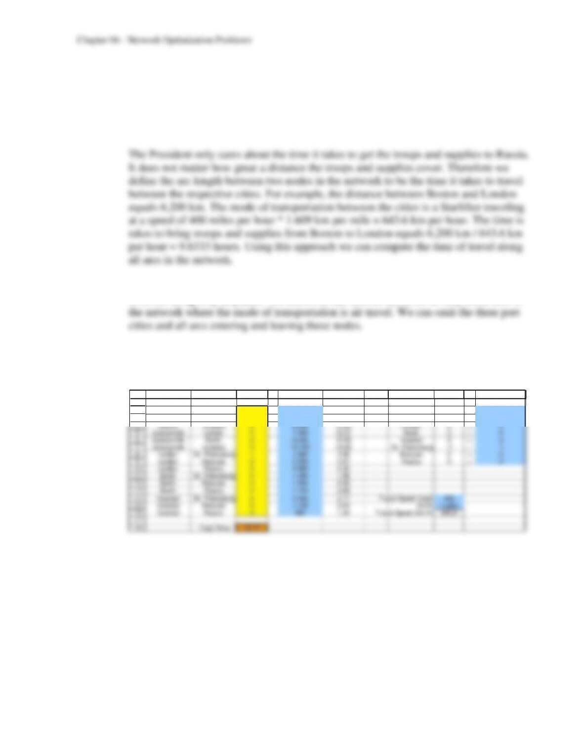
6.1 a) The network showing the different routes troops and supplies may follow to reach the
Russian Federation appears below.
Boston
Jacksonville
Napoli
Hamburg
Rotterdam
PORTS
London
AIRFIELDS
St.
Petersburg
Moscow
6-17
b) The President is only concerned about how to most quickly move troops and supplies
from the United States to the three strategic Russian cities. Obviously, the best way to
achieve this goal is to find the fastest connection between the US and the three cities.
We therefore need to find the shortest path between the US cities and each of the three
Russian cities.
By simple inspection and common sense it is apparent that the fastest transportation
involves using only airplanes. We therefore can restrict ourselves to only those arcs in
The following six spreadsheets find the shortest path between each US city (Boston and
Jacksonville) and each Russian city (St. Petersburg, Moscow, and Rostov).
Boston to St. Petersburg:
1
2
3
4
5
6
7
8
9
10
11
12
13
14
15
16
17
18
A B C D E F G H I J K
From To On Route Distance (km) Time (hou rs) Node Net F low Sup p ly/Demand
Boston London 1 6,200 9.63 Boston 1 = 1
Boston Berlin 0 7,250 11.26 Jacksonville 0 = 0
Boston Istanbul 0 8,300 12.90 London 0 = 0
Jacksonville London 0 7,900 12.27 Berlin 0 = 0
Jacksonville Berlin 0 9,200 14.29 Istanbul 0 = 0
Jacksonville Istanbul 0 10,100 15.69 St. Petersburg -1 =-1
London St. Petersburg 1 1,980 3.08 Moscow 0 = 0
London Moscow 0 2,300 3.57 Rostov 0 = 0
London Rostov 0 2,860 4.44
Berlin St. Petersburg 0 1,280 1.99
Berlin Moscow 0 1,600 2.49
Berlin Rostov 0 1,730 2.69
Istanbul St. Petersburg 0 2,040 3.17 T ravel Speed (mph) 400
Istanbul Moscow 0 1,700 2.64 km/hr 1.609
Istanbul Rostov 0 990 1.54 Travel Speed (km/hr) 643.6
Total Time 12.71