Chapter 05 – What-If Analysis for Linear Programming
5-21
f)
15
16
17
18
19
20
21
22
23
24
25
26
27
28
29
30
31
32
33
34
A B C D E F G H
Total Profit Unit Profit for W all Clocks
$1,665 $50 $100 $150 $200 $250 $300
$150 $750 $833 $1,000 $1,333 $1,667 $2,000
$200 $1,000 $1,000 $1,167 $1,333 $1,667 $2,000
Unit Profit $250 $1,250 $1,250 $1,333 $1,500 $1,667 $2,000
for Grandfather $300 $1,500 $1,500 $1,500 $1,667 $1,833 $2,000
Clocks $350 $1,750 $1,750 $1,750 $1,833 $2,000 $2,167
$400 $2,000 $2,000 $2,000 $2,000 $2,167 $2,333
$450 $2,250 $2,250 $2,250 $2,250 $2,333 $2,500
Production (G randfather Clocks, Wall Clocks) Unit Profit for W all Clocks
(3.33,3.33) $50 $100 $150 $200 $250 $300
$150 (5,0) (3.33,3.33) (3.33,3.33) (0,6.67) (0,6.67) (0,6.67)
$200 (5,0) (5,0) (3.33,3.33) (3.33,3.33) (0,6.67) (0,6.67)
Unit Profit $250 (5,0) (5,0) (3.33,3.33) (3.33,3.33) (0,6.67) (0,6.67)
for Grandfather $300 (5,0) (5,0) (5,0) (3.33,3.33) (3.33,3.33) (0,6.67)
Clocks $350 (5,0) (5,0) (5,0) (3.33,3.33) (3.33,3.33) (3.33,3.33)
$400 (5,0) (5,0) (5,0) (5,0) (3.33,3.33) (3.33,3.33)
$450 (5,0) (5,0) (5,0) (5,0) (3.33,3.33) (3.33,3.33)
g) If David increases his hours to 45 per week, the optimal solution does not change.
1
2
3
4
5
6
7
8
9
10
11
12
A B C D E F
G randfather W all
Clock Clock
Unit Profit $300 $200
Hours Hours
Used Available
Assembly (David) 6 4 33 <= 45
Carving (LaDeana) 8 4 40 <= 40
Shipping (Lydia) 3 3 20 <= 20
G randfather W all
Clock Clock Total Profit
Production 3.33 3.33 $1,667
Time Required
If LaDeana increases her hours to 45 per week, the optimal solution changes to
1
2
3
4
5
6
7
8
9
10
11
12
A B C D E F
G randfather W all
Clock Clock
Unit Profit $300 $200
Hours Hours
Used Available
Assembly (David) 6 4 36 <= 40
Carving (LaDeana) 8 4 45 <= 45
Shipping (Lydia) 3 3 20 <= 20
G randfather W all
Clock Clock Total Profit
Production 4.58 2.08 $1,792
Time Required
5-22
If Lydia increases her hours to 25 per week, the optimal solution changes to
1
2
3
4
5
6
7
8
9
10
11
12
A B C D E F
G randfather W all
Clock Clock
Unit Profit $300 $200
Hours Hours
Used Available
Assembly (David) 6 4 37 <= 40
Carving (LaDeana) 8 4 40 <= 40
Shipping (Lydia) 3 3 25 <= 25
G randfather W all
Clock Clock Total Profit
Production 1.67 6.67 $1,833
Time Required
h)
15
16
17
18
19
20
21
22
23
24
25
26
27
28
29
30
31
32
33
34
35
36
37
38
39
40
41
42
43
44
45
46
47
48
A B C D
Assembly Hours
Available Grandfather W all
(David) Clock Clock Total Profit
3.33 3.33 $1,667
35 3.33 3.33 $1,667
37 3.33 3.33 $1,667
39 3.33 3.33 $1,667
41 3.33 3.33 $1,667
43 3.33 3.33 $1,667
45 3.33 3.33 $1,667
Carving Hours
Available Grandfather W all
(LaDeana) Clock Clock Total Profit
3.33 3.33 $1,667
35 2.08 4.58 $1,542
37 2.58 4.08 $1,592
39 3.08 3.58 $1,642
41 3.58 3.08 $1,692
43 4.08 2.58 $1,742
45 4.58 2.08 $1,792
Shipping Hours
Available Grandfather W all
(Lydia) Clock Clock Total Profit
3.33 3.33 $1,667
15 5.00 0.00 $1,500
17 4.33 1.33 $1,567
19 3.67 2.67 $1,633
21 3.00 4.00 $1,700
23 2.33 5.33 $1,767
25 1.67 6.67 $1,833
5-23
i) The allowable range for the unit profit for the grandfather clock is $200 to $400.
Variable Cells
F in al Red uced O bjective Allow ab le Al low able
Cell Name Valu e Cost Coefficient Increase Decrease
$B$12 Production Clock 3.33 0.00 300 100 100
$C$12 Production Clock 3.33 0.00 200 100 50
Constraints
F in al Sh ad ow Co nstrai nt Allo w ab le Allow ab le
Cell Name Valu e Price R.H. Side Increase Decrease
$D$6 Assembly (David) Used 33 040 1E+ 30 6.667
$D$7 Carving (LaDeana) Used 40 25 40 13.333 13.333
$D$8 Shipping (Lydia) Used 20 33.33 20 10 5
j) Lydia should increase her hours slightly since her hours have the highest shadow price.
m) Percentage of Lydia’s available increase used = (25 – 20)/10 = 50%.
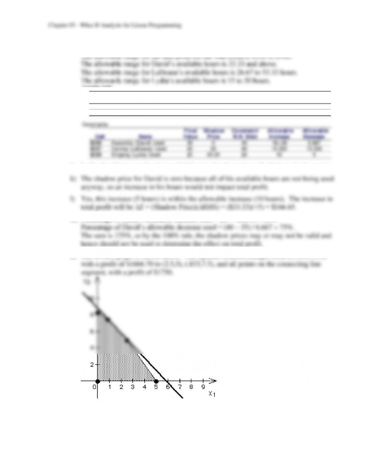
n) The revised graph is shown below. The optimal solution changes from (3.333,3.333)
5-24
5.11 a)
1
2
3
4
5
6
7
8
9
10
11
A B C D E F
Toys Subassemblies
Unit Profit $3.00 -$2.50
Used Available
Subassembly A 2 -1 3,000 <= 3,000
Subassembly B 1 -1 1,000 <= 1,000
Toys Subassemblies Total Profit
Production 2,000 1,000 $3,500.00
<=
2,500
Resource Usage
b)
1
2
3
4
5
6
7
8
9
10
11
A B C D E F
Toys Subassemblies
Unit Profit $3.00 -$2.50
Used Available
Subassembly A 2 -1 3,001 <= 3,001
Subassembly B 1 -1 1,000 <= 1,000
Toys Subassemblies Total Profit
Production 2,001 1,001 $3,500.50
<=
2,500
Resource Usage
c)
1
2
3
4
5
6
7
8
9
10
11
A B C D E F
Toys Subassemblies
Unit Profit $3.00 -$2.50
Used Available
Subassembly A 2 -1 3,000 <= 3,000
Subassembly B 1 -1 1,001 <= 1,001
Toys Subassemblies Total Profit
Production 1,999 998 $3,502.00
<=
2,500
Resource Usage
5-25
d)
14
15
16
17
18
19
20
21
22
23
24
25
26
27
A B C D E
Available Total Incremental
Subassembly A Toys Subassemblies Profit Profit
2,000 1,000 $3,500.00
3,000 2,000 1,000 $3,500.00
3,100 2,100 1,100 $3,550.00 $50.00
3,200 2,200 1,200 $3,600.00 $50.00
3,300 2,300 1,300 $3,650.00 $50.00
3,400 2,400 1,400 $3,700.00 $50.00
3,500 2,500 1,500 $3,750.00 $50.00
3,600 2,500 1,500 $3,750.00 $0.00
3,700 2,500 1,500 $3,750.00 $0.00
3,800 2,500 1,500 $3,750.00 $0.00
3,900 2,500 1,500 $3,750.00 $0.00
4,000 2,500 1,500 $3,750.00 $0.00
Production
e)
14
15
16
17
18
19
20
21
22
23
24
25
26
27
A B C D E
Available Total Incremental
Subassembly B Toys Subassemblies Profit Profit
2,000 1,000 $3,500.00
1,000 2,000 1,000 $3,500.00
1,100 1,900 800 $3,700.00 $200.00
1,200 1,800 600 $3,900.00 $200.00
1,300 1,700 400 $4,100.00 $200.00
1,400 1,600 200 $4,300.00 $200.00
1,500 1,500 0 $4,500.00 $200.00
1,600 1,500 0 $4,500.00 $0.00
1,700 1,500 0 $4,500.00 $0.00
1,800 1,500 0 $4,500.00 $0.00
1,900 1,500 0 $4,500.00 $0.00
2,000 1,500 0 $4,500.00 $0.00
Production
f)
Variable Cells
Final Reduced Objective Allowable Allowable
Cell Name Value Cost Coefficient Increase Decrease
$B$9 Production Toys 2,000 0 3 2 0.5
$C$9 Production Subassemblies 1,000 0 -2.5 1 0.5
Constraints
Final Shadow Constraint Allowable Allo wable
Cell Name Value Price R.H. Side Increase Decrease
$D$5 Subassembly A Used 3,000 0.5 3000 500 1000
$D$6 Subassembly B Used 1,000 2 1000 500 500
As shown in the sensitivity report, the shadow price is $0.50 for subassembly A is
$2.00 for subassembly B. According to the allowable increase and allowable decrease,
5.12 a) The original model:
1
2
3
4
5
6
7
8
9
A B C D E F
Activity 1 Activity 2
Unit Profit $2 $5
Used Available
Resource 1 1 2 10 <= 10
Resource 2 1 3 12 <= 12
Activity 1 Activity 2 Total Profit
Solution 6 2 $22.00
Resource Usage
With 1 additional unit of resource 1:
1
2
3
4
5
6
7
8
9
A B C D E F
Activity 1 Activity 2
Unit Profit $2 $5
Used Available
Resource 1 1 2 11 <= 11
Resource 2 1 3 12 <= 12
Activity 1 Activity 2 Total Profit
Solution 9 1 $23.00
Resource Usage
5-27
b)
12
13
14
15
16
17
18
19
20
21
22
23
24
25
A B C D E
Available Total Incremental
Resource 1 Activity 1 Activity 2 Profit Profit
6 2 $22.00
5 0 2.5 $12.50
6 0 3 $15.00 $2.50
7 0 3.5 $17.50 $2.50
8 0 4 $20.00 $2.50
9 3 3 $21.00 $1.00
10 6 2 $22.00 $1.00
11 9 1 $23.00 $1.00
12 12 0 $24.00 $1.00
13 12 0 $24.00 $0.00
14 12 0 $24.00 $0.00
15 12 0 $24.00 $0.00
Solution
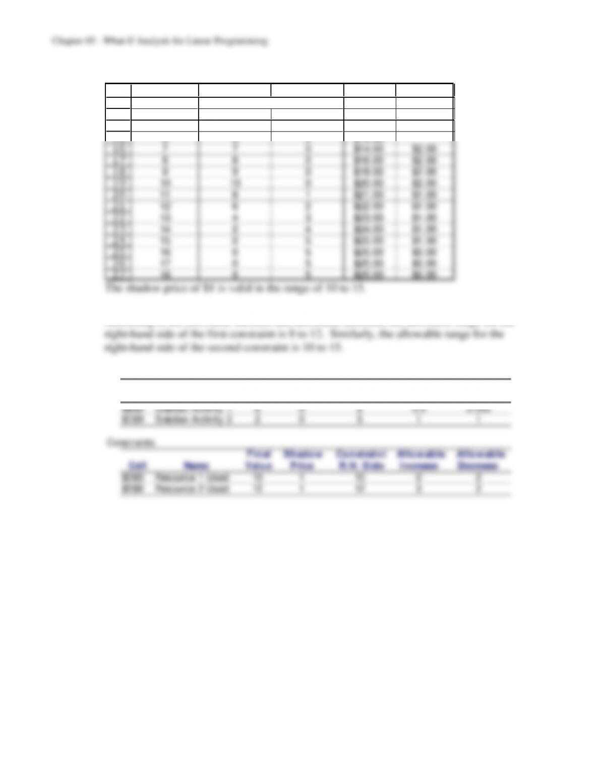
The shadow price of $1 is valid in the range of 8 to 12.
c) With 1 additional unit of resource 2:
1
2
3
4
5
6
7
8
9
A B C D E F
Activity 1 Activity 2
Unit Profit $2 $5
Used Available
Resource 1 1 2 10 <= 10
Resource 2 1 3 13 <= 13
Activity 1 Activity 2 Total Profit
Solution 4 3 $23.00
Resource Usage
5-28
d)
12
13
14
15
16
17
18
19
20
21
22
23
24
25
26
27
18 0 5 $25.00 $0.00
A B C D E
Available Total Incremental
Resource 2 Activity 1 Activity 2 Profit Profit
6 2 $22.00
6 6 0 $12.00
7 7 0 $14.00 $2.00
8 8 0 $16.00 $2.00
9 9 0 $18.00 $2.00
10 10 0 $20.00 $2.00
11 8 1 $21.00 $1.00
12 6 2 $22.00 $1.00
13 4 3 $23.00 $1.00
14 2 4 $24.00 $1.00
15 0 5 $25.00 $1.00
16 0 5 $25.00 $0.00
17 0 5 $25.00 $0.00
Solution
e) As shown in the sensitivity report, the shadow prices for both constraints are $1.
According to the allowable increase and allowable decrease, the allowable range for the
Variable Cells
Final Reduced O bjective Allo wable Allowable
Cell Name Valu e Cost Coefficient Increase Decrease
$B$9 Solution Activity 1 6 0 2 0.5 0.333
$C$9 Solution Activity 2 2 0 5 1 1
Constraints
Final Shadow Constraint Allowable Allo wable
Cell Name Valu e Price R.H. Side Increase Decrease
$D$5 Resource 1 Used 10 110 2 2
$D$6 Resource 2 Used 12 112 3 2
5-29
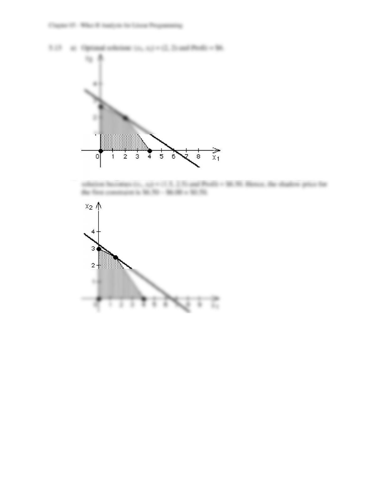
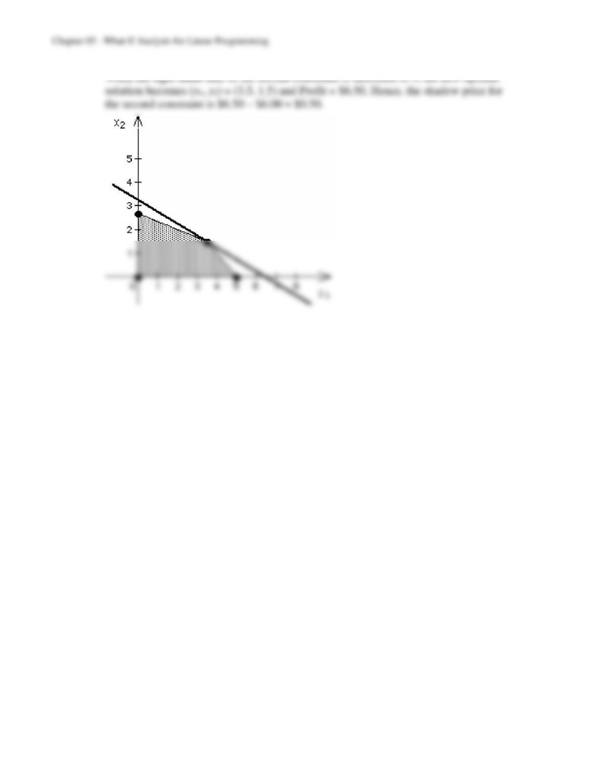
b) When the right-hand-side of the first constraint is increased to 9, the new optimal
5-30
5-31
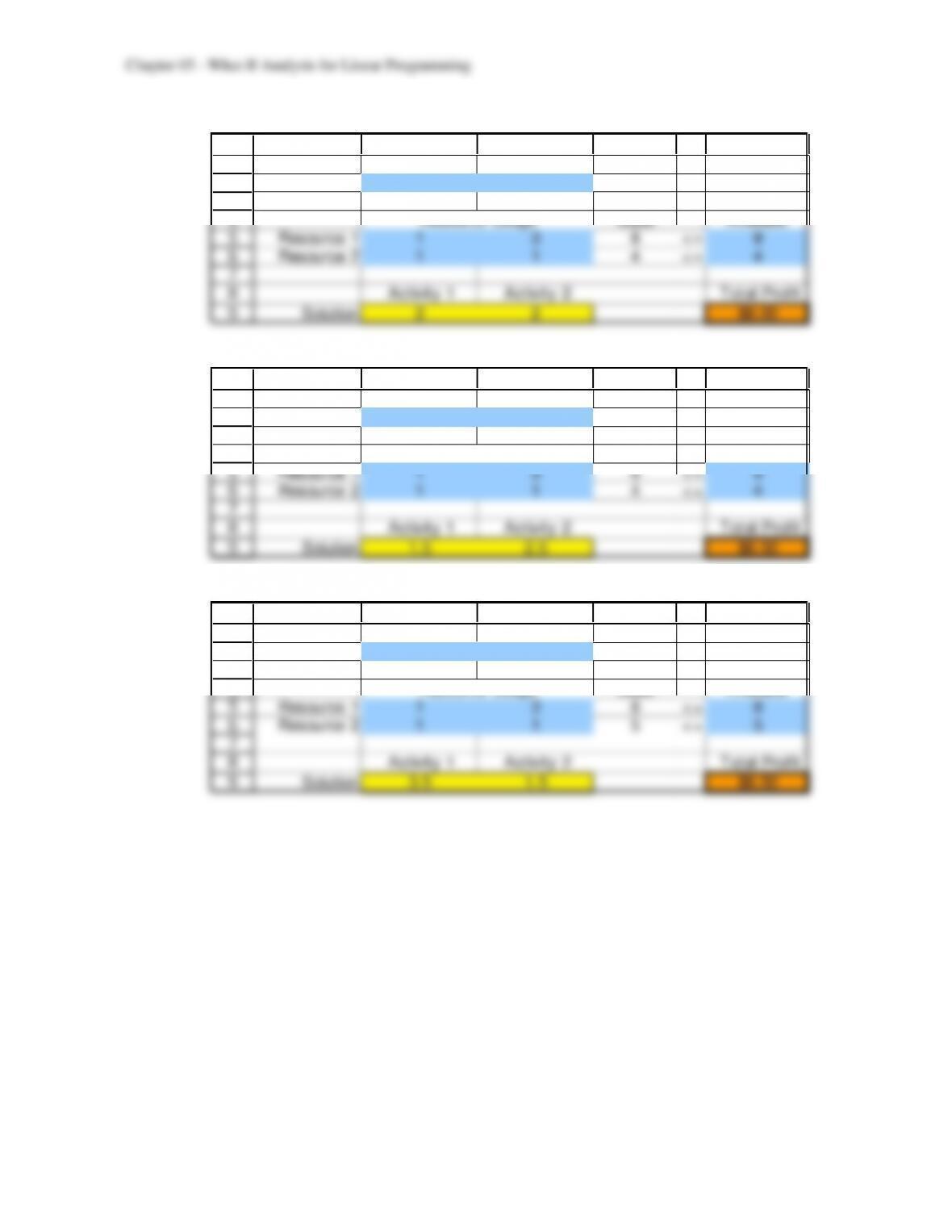
c) Original model:
1
2
3
4
5
6
7
8
9
A B C D E F
Activity 1 Activity 2
Unit Profit $1 $2
Used Available
Resource 1 1 3 8 <= 8
Resource 2 1 1 4 <= 4
Activity 1 Activity 2 Total Profit
Solution 2 2 $6.00
Resource Usage
The shadow price for resource 1 is $0.50.
1
2
3
4
5
6
7
8
9
A B C D E F
Activity 1 Activity 2
Unit Profit $1 $2
Used Available
Resource 1 1 3 9 <= 9
Resource 2 1 1 4 <= 4
Activity 1 Activity 2 Total Profit
Solution 1.5 2.5 $6.50
Resource Usage
The shadow price for resource 2 is $0.50.
1
2
3
4
5
6
7
8
9
A B C D E F
Activity 1 Activity 2
Unit Profit $1 $2
Used Available
Resource 1 1 3 8 <= 8
Resource 2 1 1 5 <= 5
Activity 1 Activity 2 Total Profit
Solution 3.5 1.5 $6.50
Resource Usage
5-32
d) The allowable range for the right-hand side of the resource 1 constraint is
approximately from 4 (or less) to 12.
12
13
14
15
16
17
18
19
20
21
22
23
24
25
A B C D E
Available Total Incremental
Resource 1 Activity 1 Activity 2 Profit Profit
2 2 $6.00
4 4 0 $4.00
5 3.5 0.5 $4.50 $0.50
6 3 1 $5.00 $0.50
7 2.5 1.5 $5.50 $0.50
8 2 2 $6.00 $0.50
9 1.5 2.5 $6.50 $0.50
10 1 3 $7.00 $0.50
11 0.5 3.5 $7.50 $0.50
12 0 4 $8.00 $0.50
13 0 4 $8.00 $0.00
14 0 4 $8.00 $0.00
Solution
The allowable range for the right-hand side of the resource 2 constraint is
approximately from 3 to 8.
28
29
30
31
32
33
34
35
36
37
38
39
40
41
A B C D E
Available Total Incremental
Resource 2 Activity 1 Activity 2 Profit Profit
2 2 $6.00
0 0 0 $0.00
1 0 1 $2.00 $2.00
2 0 2 $4.00 $2.00
3 0.5 2.5 $5.50 $1.50
4 2 2 $6.00 $0.50
5 3.5 1.5 $6.50 $0.50
6 5 1 $7.00 $0.50
7 6.5 0.5 $7.50 $0.50
8 8 0 $8.00 $0.50
9 8 0 $8.00 $0.00
10 8 0 $8.00 $0.00
Solution
Variable Cells
Final Reduced Objective Allo w able Allo w able
Cell Name Value Cost Coefficient Increase Decrease
$B$9 Solution Activity 1 2 0 1 1 0.333
$C$9 Solution Activity 2 2 0 2 1 1
Constraints
Final Shado w Constraint Allowable Allowable
Cell Name Value Price R.H. Side Increase Decrease
$D$5 Resource 1 Used 8 0.5 8 4 4
$D$6 Resource 2 Used 4 0.5 4 4 1.333
5-33
5.14 a) Optimal solution: (x1, x2) = (3, 4) and Profit = $17.
b) When the right-hand-side of the first constraint is increased to 5, the optimal solution
remains the same. Hence, the shadow price for the first constraint is 0.
5-34
When the right-hand-side of the second constraint is increased to 16, the new optimal
When the right-hand-side of the third constraint is increased to 11, the new optimal
5-35
c) Original model:
1
2
3
4
5
6
7
8
9
10
A B C D E F
Activity 1 Activity 2
Unit Profit $3 $2
Used Available
Resource 1 1 0 3 <= 4
Resource 2 1 3 15 <= 15
Resource 3 2 1 10 <= 10
Activity 1 Activity 2 Total Profit
Solution 3 4 $17.00
Resource Usage
The shadow price for resource 1 is $0.
1
2
3
4
5
6
7
8
9
10
A B C D E F
Activity 1 Activity 2
Unit Profit $3 $2
Used Available
Resource 1 1 0 3 <= 5
Resource 2 1 3 15 <= 15
Resource 3 2 1 10 <= 10
Activity 1 Activity 2 Total Profit
Solution 3 4 $17.00
Resource Usage
The shadow price for resource 2 is $0.20.
1
2
3
4
5
6
7
8
9
10
A B C D E F
Activity 1 Activity 2
Unit Profit $3 $2
Used Available
Resource 1 1 0 2.8 <= 4
Resource 2 1 3 16 <= 16
Resource 3 2 1 10 <= 10
Activity 1 Activity 2 Total Profit
Solution 2.8 4.4 $17.20
Resource Usage
The shadow price for resource 3 is $1.40.
1
2
3
4
5
6
7
8
9
10
A B C D E F
Activity 1 Activity 2
Unit Profit $3 $2
Used Available
Resource 1 1 0 3.6 <= 4
Resource 2 1 3 15 <= 15
Resource 3 2 1 11 <= 11
Activity 1 Activity 2 Total Profit
Solution 3.6 3.8 $18.40
Resource Usage
5-36
d) The allowable range for the right-hand side of the resource 1 constraint is
approximately from 3 to at least 10.
13
14
15
16
17
18
19
20
21
22
23
24
25
26
A B C D E
Available Total Incremental
Resource 1 Activity 1 Activity 2 Profit Profit
3 4 $17.00
0 0 5 $10.00
1 1 4.667 $12.33 $2.33
2 2 4.333 $14.67 $2.33
3 3 4 $17.00 $2.33
4 3 4 $17.00 $0.00
5 3 4 $17.00 $0.00
6 3 4 $17.00 $0.00
7 3 4 $17.00 $0.00
8 3 4 $17.00 $0.00
9 3 4 $17.00 $0.00
10 3 4 $17.00 $0.00
Solution
The allowable range for the right-hand side of the resource 2 constraint is
approximately from less than 11 to more than 21.
29
30
31
32
33
34
35
36
37
38
39
40
41
42
A B C D E
Available Total Incremental
Resource 2 Activity 1 Activity 2 Profit Profit
3 4 $17.00
11 3.8 2.4 $16.20
12 3.6 2.8 $16.40 $0.20
13 3.4 3.2 $16.60 $0.20
14 3.2 3.6 $16.80 $0.20
15 3 4 $17.00 $0.20
16 2.8 4.4 $17.20 $0.20
17 2.6 4.8 $17.40 $0.20
18 2.4 5.2 $17.60 $0.20
19 2.2 5.6 $17.80 $0.20
20 2 6 $18.00 $0.20
21 1.8 6.4 $18.20 $0.20
Solution
5-38
5.15
3
4
5
6
7
8
9
10
11
12
13
14
15
B C D E F G H
TV Spots Magazine Ads SS Ads
Exposures per Ad 1,300 600 500
(thousands)
Budget Budget
Cost per Ad ($thousands) Spent Available
Ad Budget 300 150 100 4,000 <= 4,000
Planning Budget 90 30 40 1,000 <= 1,000
Total Exposures
TV Spots Magazine Ads SS Ads (thousands)
Number of Ads 0 20 10 17,000
<=
Max TV Spots 5
Variable Cells
Final Reduced Objective Allowable Allowable
Cell Name Valu e Cost Coefficient Increase Decrease
$C$13 TVSpots 0 -50 1300 50 1E+ 30
$D$13 Number of Ads Magazine Ads 20 0 600 150 50
$E$13 Number of Ads SS Ads 10 0 500 300 33.333
Constraints
Final Shadow Constraint Allowable Allowable
Cell Name Valu e Price R.H. Side Increase Decrease
$F$8 Ad Budget Spent 4,000 3 4000 1000 1500
$F$9 Planning Budget Spent 1,000 5 1000 600 200
a) The total number of expected exposures could be increased by 3,000 for each additional
d) This remains valid for increases of up to $600,000.
e) Percentage of allowable increase for ad budget = (4,100 – 4,000) / 1,000 = 10%
f) The $100,000 should be added to the planning budget since this will add 500,000
5-39
5.16
3
4
5
6
7
8
9
10
11
12
13
14
15
16
17
18
19
20
21
B C D E F G H
TV Spots Magazine Ads SS Ads
Exposures per Ad 1,300 600 500
(thousands)
Cost per Ad ($thousands) Budget Spent Budget Available
Ad Budget 300 150 100 3,775 <= 4,000
Planning Budget 90 30 40 1,000 <= 1,000
Number Reached per Ad (millions) Total Reached Minimum Acceptable
Young Children 1.2 0.1 0 5 >= 5
Parents of Young Children 0.5 0.2 0.2 5.85 >= 5
TV Spots Magazine Ads SS Ads Total Redeemed Required Amount
Coupon Redemption per Ad 0 40 120 1,490 = 1,490
($thousands)
Total Exposures
TV Spots Magazine Ads SS Ads (thousands)
Number of Ads 3 14 7.75 16,175
<=
Maximum TV Spots 5
Variable Cells
Final Redu ced Objective Allowable Allowable
Cell Name Value Cost Coefficient Increase Decrease
$C$19 TVSpots 3 0 1300 1040 1E+ 30
$D$19 Number of Ads Magazine Ads 14 0 600 1E+ 30 192.59
$E$19 Number of Ads SS Ads 7.75 0 500 577.78 1E+ 30
Constraints
Final Shadow Constraint Allowable Allowable
Cell Name Value Price R.H. Side Increase Decrease
$F$7 Ad Budget Budget Spent 3,775 0 4000 1E+ 30 225
$F$8 Planning Budget Budget Spent 1,000 35 1000 22.5 85
$F$15 TotalRedeemed 1,490 -8 1490 385 90
$F$11 Young Children Total Reached 5 -1575.76 5 1.32 0.45
$F$12 Parents of Young Children Total Reached 5.85 0 5 0.85 1E+ 30
a) The total number of expected exposures can not be increased by adding an additional
d) This remains valid for increases of up to $22,500.
f) $100,000 is beyond the allowable increase for the planning budget. Therefore, the total