5-1
Chapter 5 What-If Analysis for Linear Programming
Review Questions
5.1-1 The parameters of a linear programming model are the constants (coefficients or right-hand
sides) in the functional constraints and the objective function.
5.1-2 Many of the parameters of a linear programming model are only estimates of quantities that
cannot be determined precisely and thus result in inaccuracies.
5.1-4 No, if the optimal solution will remain the same over a wide range of values for a particular
coefficient, then it may be appropriate to make only a fairly rough estimate for a parameter
of a model.
5.1-5 Conditions that impact the parameters of a model, such as unit profit, may change over
time and render them inaccurate.
5.1-8 What-if analysis provides guidance about what the impact would be of altering policy
decisions that are represented by parameters of a model.
5.2-1 The estimates of the unit profits for the two products are most questionable.
5.2-2 The number of hours of production time that is being made available per week in the three
plants might change after analysis.
5.3-3 The Objective Coefficient column gives the current value of each coefficient. The
Allowable Increase column and the Allowable Decrease Column give the amount that each
coefficient may differ from these values to remain within the allowable range for which the
optimal solution for the original model remains optimal.
5-3
5.6-5 The 100 percent rule basically says that we can safely use the shadow prices to predict the
effect of simultaneous changes in the right-hand sides if the sum of the percentages of the
changes does not exceed 100 percent.
5.6-7 If the sum of the percentage changes does not exceed 100%, the shadow prices definitely
will still be valid.
5.6-8 If the sum of the percentages of allowable changes in the right-hand sides does exceed
100%, then we cannot be sure if the shadow prices will still be valid.
Problems
5.1 a)
1
2
3
4
5
6
7
8
9
A B C D E F
Toys Subassemblies
Unit Profit $3.00 -$2.50
Used Available
Subassembly A 2 -1 3,000 <= 3,000
Subassembly B 1 -1 1,000 <= 1,000
Toys Subassemblies Total Profit
Production 2,000 1,000 $3,500
Resource Usage
b)
Unit
Profit
Optimal
Production Rates
Total
for Toys
Toys
Subassemblies
Profit
$2.00
1000
0
$2000
$2.50
1000
0
$2500
$3.00
2000
1000
$3500
$3.50
2000
1000
$4500
$4.00
2000
1000
$5500
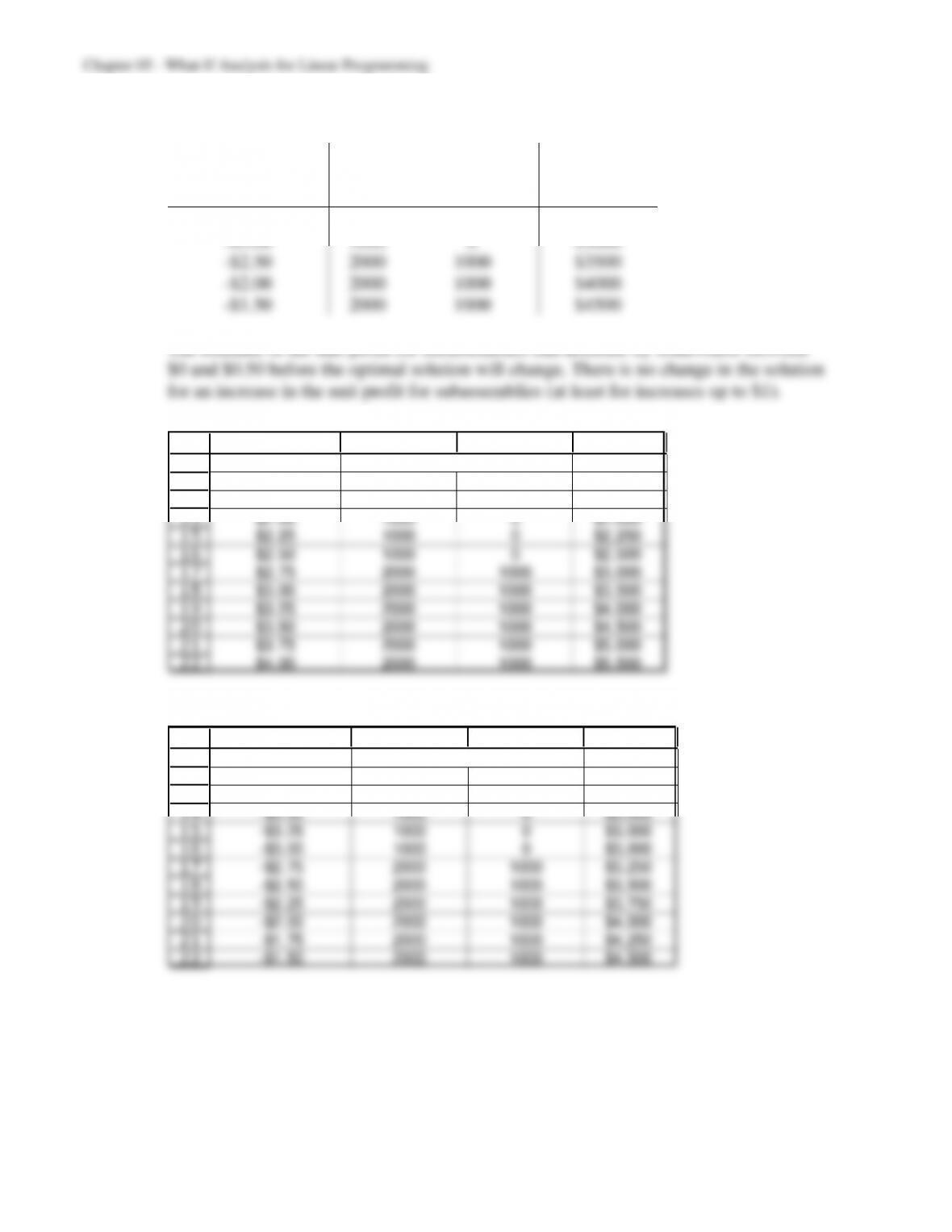
The estimate of the unit profit for toys can decrease by somewhere between $0 and
5-4
c)
Unit Profit
Optimal
Production Rates
Total
for Subassemblies
Toys
Subassemblies
Profit
-$3.50
1000
0
$3000
-$3.00
1000
0
$3000
-$2.50
2000
1000
$3500
-$2.00
2000
1000
$4000
-$1.50
2000
1000
$4500
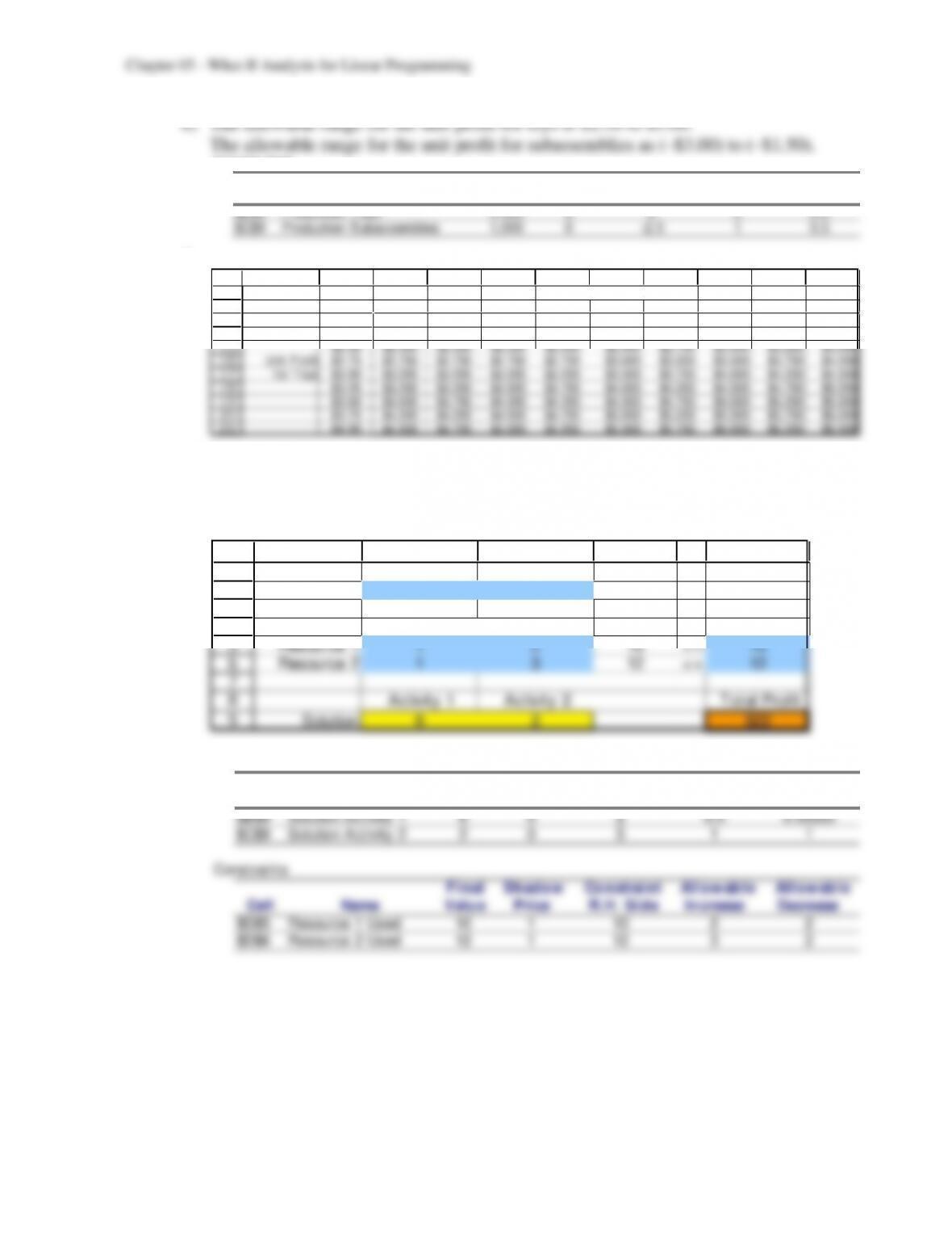
The estimate of the unit profit for subassemblies can decrease by somewhere between
d) Solver Table for change in unit profit for toys (part b):
11
12
13
14
15
16
17
18
19
20
21
22
A B C D
Unit Profit
for Toys Toys Subassemblies Total Profit
2,000 1,000 $3,500
$2.00 1000 0 $2,000
$2.25 1000 0 $2,250
$2.50 1000 0 $2,500
$2.75 2000 1000 $3,000
$3.00 2000 1000 $3,500
$3.25 2000 1000 $4,000
$3.50 2000 1000 $4,500
$3.75 2000 1000 $5,000
$4.00 2000 1000 $5,500
Production
Solver Table for change in unit profit for subassemblies (part c):
11
12
13
14
15
16
17
18
19
20
21
22
A B C D
Unit Profit
for Subassemblies Toys Subassemblies Total Profit
2,000 1,000 $3,500
-$3.50 1000 0 $3,000
-$3.25 1000 0 $3,000
-$3.00 1000 0 $3,000
-$2.75 2000 1000 $3,250
-$2.50 2000 1000 $3,500
-$2.25 2000 1000 $3,750
-$2.00 2000 1000 $4,000
-$1.75 2000 1000 $4,250
-$1.50 2000 1000 $4,500
Production
5-5
Variable Cells
Final Reduced Ob jective Allowable Allowable
Cell Name Value Cost Coefficient Increase Decrease
$B$9 Production Toys 2,000 0 3 2 0.5
$C$9 Production Subassemblies 1,000 0 -2.5 1 0.5
f)
11
12
13
14
15
16
17
18
19
20
21
$4.00 $4,500 $4,750 $5,000 $5,250 $5,500 $5,750 $6,000 $6,250 $6,500
A B C D E F G H I J K
Total Profit Unit Profit for Subassemblies
$3,500 -$3.50 -$3.25 -$3.00 -$2.75 -$2.50 -$2.25 -$2.00 -$1.75 -$1.50
$2.00 $2,000 $2,000 $2,000 $2,000 $2,000 $2,000 $2,000 $2,250 $2,500
$2.25 $2,250 $2,250 $2,250 $2,250 $2,250 $2,250 $2,500 $2,750 $3,000
$2.50 $2,500 $2,500 $2,500 $2,500 $2,500 $2,750 $3,000 $3,250 $3,500
Unit Profit $2.75 $2,750 $2,750 $2,750 $2,750 $3,000 $3,250 $3,500 $3,750 $4,000
for Toys $3.00 $3,000 $3,000 $3,000 $3,250 $3,500 $3,750 $4,000 $4,250 $4,500
$3.25 $3,250 $3,250 $3,500 $3,750 $4,000 $4,250 $4,500 $4,750 $5,000
$3.50 $3,500 $3,750 $4,000 $4,250 $4,500 $4,750 $5,000 $5,250 $5,500
$3.75 $4,000 $4,250 $4,500 $4,750 $5,000 $5,250 $5,500 $5,750 $6,000
g) So long as the sum of the percentage change of the unit profit for the subassemblies
does not exceed 100% (where the allowable increase and decrease are given in part f),
then the solution will not change.
5.2 a)
1
2
3
4
5
6
7
8
9
A B C D E F
Activity 1 Activity 2
Unit Profit $2 $5
Used Available
Resource 1 1 2 10 <= 10
Resource 2 1 3 12 <= 12
Activity 1 Activity 2 Total Profit
Solution 6 2 $22
Resource Usage
Variable Cells
F in al Redu ced O bjective All ow abl e Allow able
Cell Name Valu e Cost Coefficient Increase Decrease
$B$9 Solution Activity 1 6 0 2 0.5 0.33333
$C$9 Solution Activity 2 2 0 5 1 1
Constraints
F in al Sh ad ow Con straint Allow able Allow able
Cell Name Valu e Price R.H. Side Increase Decrease
$D$5 Resource 1 Used 10 110 2 2
$D$6 Resource 2 Used 12 112 3 2
5-6
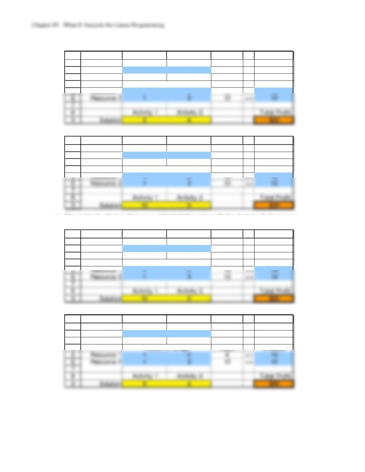
b) The optimal solution changes to (0, 4) if the unit profit for Activity 1 changes to $1.
1
2
3
4
5
6
7
8
9
A B C D E F
Activity 1 Activity 2
Unit Profit $1 $5
Used Available
Resource 1 1 2 8 <= 10
Resource 2 1 3 12 <= 12
Activity 1 Activity 2 Total Profit
Solution 0 4 $20
Resource Usage
The optimal solution changes to (10, 0) if the unit profit for Activity 1 changes to $3.
1
2
3
4
5
6
7
8
9
A B C D E F
Activity 1 Activity 2
Unit Profit $3 $5
Used Available
Resource 1 1 2 10 <= 10
Resource 2 1 3 10 <= 12
Activity 1 Activity 2 Total Profit
Solution 10 0 $30
Resource Usage
c) The optimal solution changes to (10, 0) if the unit profit for Activity 2 changes to
$2.50.
1
2
3
4
5
6
7
8
9
A B C D E F
Activity 1 Activity 2
Unit Profit $2 $2.50
Used Available
Resource 1 1 2 10 <= 10
Resource 2 1 3 10 <= 12
Activity 1 Activity 2 Total Profit
Solution 10 0 $20
Resource Usage
The optimal solution changes to (0, 4) if the unit profit for Activity 2 changes to $7.50.
1
2
3
4
5
6
7
8
9
A B C D E F
Activity 1 Activity 2
Unit Profit $2 $7.50
Used Available
Resource 1 1 2 8 <= 10
Resource 2 1 3 12 <= 12
Activity 1 Activity 2 Total Profit
Solution 0 4 $30
Resource Usage
5-7
d)
11
12
13
14
15
16
17
18
19
20
21
22
23
24
25
26
27
28
29
30
31
32
33
34
35
36
37
38
39
40
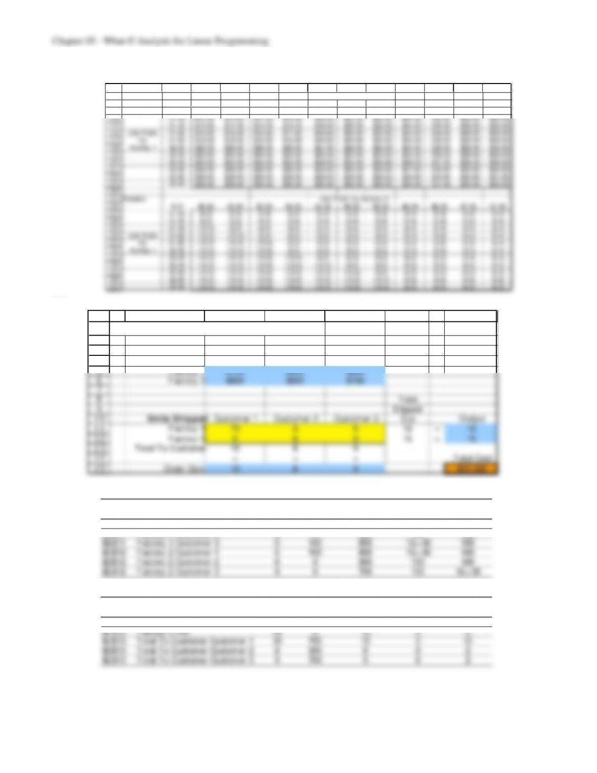
A B C D
Unit Profit for Total
Activity 1 Activity 1 Activity 2 Profit
6 2 $22.00
$1.00 0 4 $20.00
$1.20 0 4 $20.00
$1.40 0 4 $20.00
$1.60 0 4 $20.00
$1.80 6 2 $20.80
$2.00 6 2 $22.00
$2.20 6 2 $23.20
$2.40 6 2 $24.40
$2.60 10 0 $26.00
$2.80 10 0 $28.00
$3.00 10 0 $30.00
Unit Profit for Total
Activity 2 Activity 1 Activity 2 Profit
6 2 $22.00
$2.50 10 0 $20.00
$3.00 10 0 $20.00
$3.50 10 0 $20.00
$4.00 6 2 $20.00
$4.50 6 2 $21.00
$5.00 6 2 $22.00
$5.50 6 2 $23.00
$6.00 0 4 $24.00
$6.50 0 4 $26.00
$7.00 0 4 $28.00
$7.50 0 4 $30.00
Solution
Solution
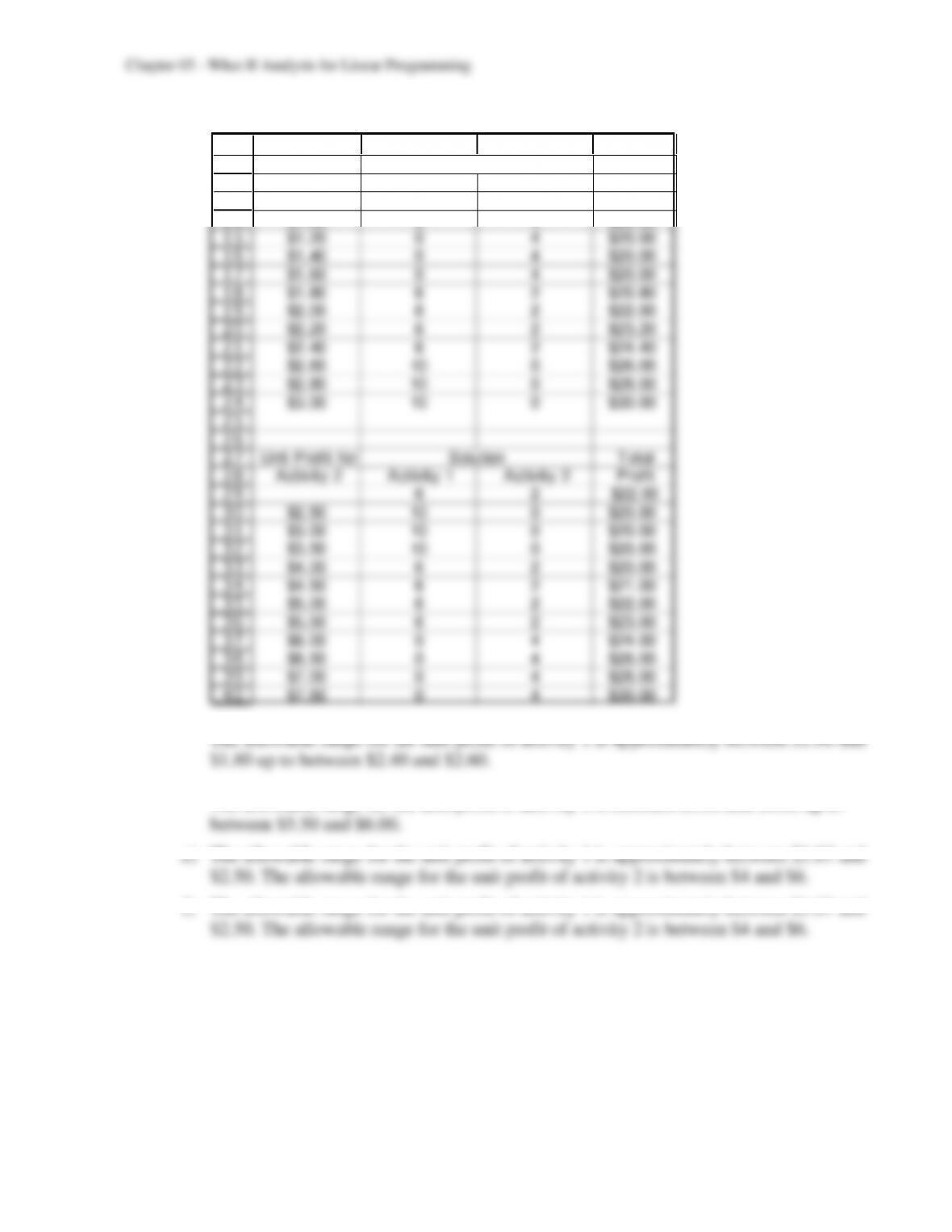
The allowable range for the unit profit of activity 2 is between $3.50 and $4.00 up to
f) The allowable range for the unit profit of activity 1 is approximately between $1.67 and
5-8
g)
11
12
13
14
15
16
17
18
19
20
21
22
23
24
25
26
27
28
29
30
31
32
33
34
35
36
37
A B C D E F G H I J K L M
Total Profit Unit Profit for Activity 2
$22 $2.50 $3.00 $3.50 $4.00 $4.50 $5.00 $5.50 $6.00 $6.50 $7.00 $7.50
$1.00 $11.00 $12.00 $14.00 $16.00 $18.00 $20.00 $22.00 $24.00 $26.00 $28.00 $30.00
$1.20 $12.20 $13.20 $14.20 $16.00 $18.00 $20.00 $22.00 $24.00 $26.00 $28.00 $30.00
$1.40 $14.00 $14.40 $15.40 $16.40 $18.00 $20.00 $22.00 $24.00 $26.00 $28.00 $30.00
Unit Profit $1.60 $16.00 $16.00 $16.60 $17.60 $18.60 $20.00 $22.00 $24.00 $26.00 $28.00 $30.00
for $1.80 $18.00 $18.00 $18.00 $18.80 $19.80 $20.80 $22.00 $24.00 $26.00 $28.00 $30.00
Activity 1 $2.00 $20.00 $20.00 $20.00 $20.00 $21.00 $22.00 $23.00 $24.00 $26.00 $28.00 $30.00
$2.20 $22.00 $22.00 $22.00 $22.00 $22.20 $23.20 $24.20 $25.20 $26.20 $28.00 $30.00
$2.40 $24.00 $24.00 $24.00 $24.00 $24.00 $24.40 $25.40 $26.40 $27.40 $28.40 $30.00
$2.60 $26.00 $26.00 $26.00 $26.00 $26.00 $26.00 $26.60 $27.60 $28.60 $29.60 $30.60
$2.80 $28.00 $28.00 $28.00 $28.00 $28.00 $28.00 $28.00 $28.80 $29.80 $30.80 $31.80
$3.00 $30.00 $30.00 $30.00 $30.00 $30.00 $30.00 $30.00 $30.00 $31.00 $32.00 $33.00
Solution Unit Profit for Activity 2
(6,2) $2.50 $3.00 $3.50 $4.00 $4.50 $5.00 $5.50 $6.00 $6.50 $7.00 $7.50
$1.00 (6,2) (0,4) (0,4) (0,4) (0,4) (0,4) (0,4) (0,4) (0,4) (0,4) (0,4)
$1.20 (6,2) (6,2) (6,2) (0,4) (0,4) (0,4) (0,4) (0,4) (0,4) (0,4) (0,4)
$1.40 (10,0) (6,2) (6,2) (6,2) (0,4) (0,4) (0,4) (0,4) (0,4) (0,4) (0,4)
Unit Profit $1.60 (10,0) (10,0) (6,2) (6,2) (6,2) (0,4) (0,4) (0,4) (0,4) (0,4) (0,4)
for $1.80 (10,0) (10,0) (10,0) (6,2) (6,2) (6,2) (0,4) (0,4) (0,4) (0,4) (0,4)
Activity 1 $2.00 (10,0) (10,0) (10,0) (6,2) (6,2) (6,2) (6,2) (0,4) (0,4) (0,4) (0,4)
$2.20 (10,0) (10,0) (10,0) (10,0) (6,2) (6,2) (6,2) (6,2) (6,2) (0,4) (0,4)
$2.40 (10,0) (10,0) (10,0) (10,0) (10,0) (6,2) (6,2) (6,2) (6,2) (6,2) (0,4)
$2.60 (10,0) (10,0) (10,0) (10,0) (10,0) (10,0) (6,2) (6,2) (6,2) (6,2) (6,2)
$2.80 (10,0) (10,0) (10,0) (10,0) (10,0) (10,0) (10,0) (6,2) (6,2) (6,2) (6,2)
$3.00 (10,0) (10,0) (10,0) (10,0) (10,0) (10,0) (10,0) (6,2) (6,2) (6,2) (6,2)
5.3
1
2
3
4
5
6
7
8
9
10
11
12
13
14
15
A B C D E F G H
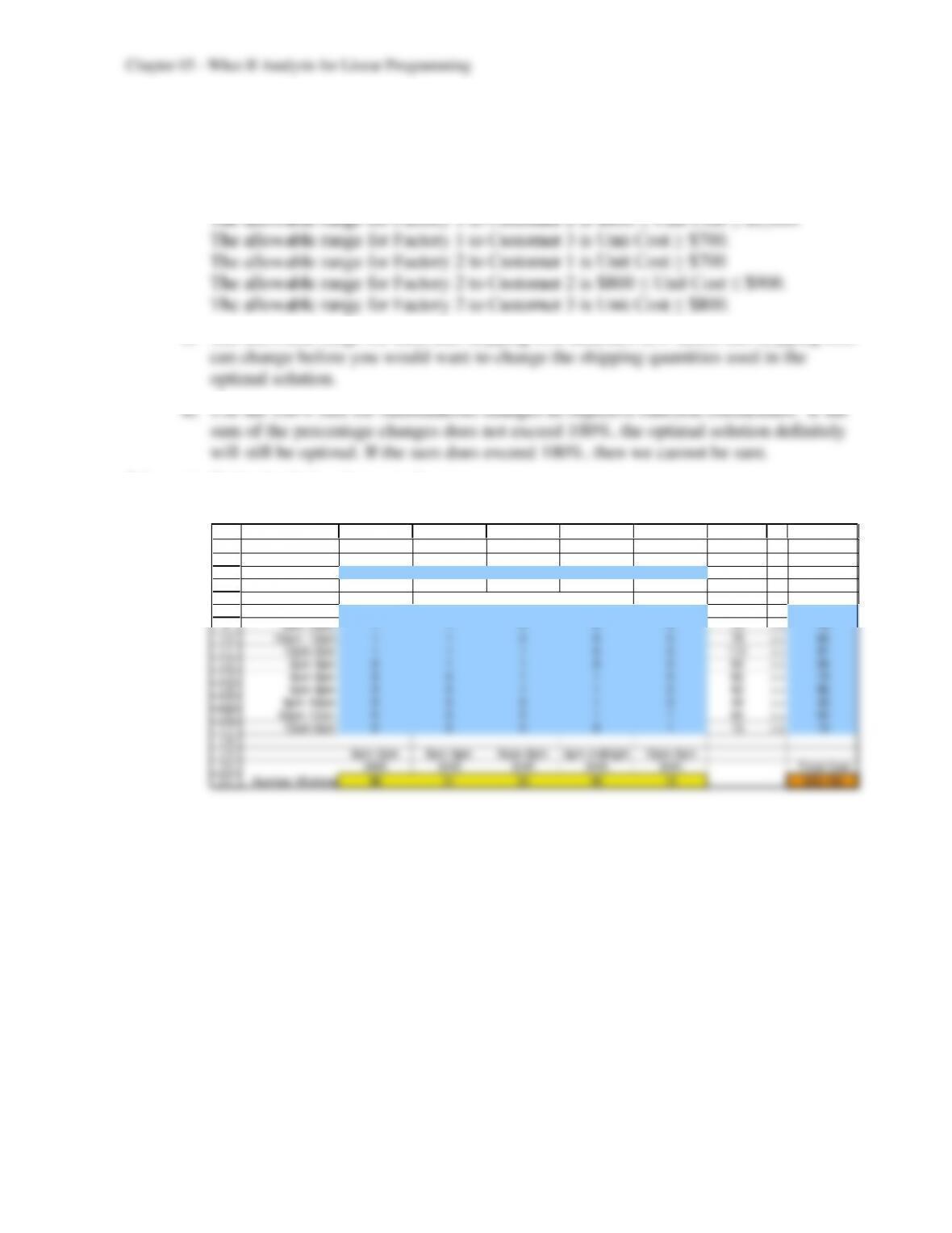
Big M Company Distribution Problem
Ship ping Cost
(p er Lathe) Customer 1 Customer 2 Customer 3
Factory 1 $700 $900 $800
Factory 2 $800 $900 $700
Total
Shipped
Units Shipp ed Customer 1 Customer 2 Customer 3 Out Output
Factory 1 10 2 0 12 =12
Factory 2 0 6 9 15 =15
Total To Customer 10 8 9
= = = Total Cost
Order Size 10 8 9 $20,500
Variable Cells
F in al Redu ced O bjective Allo w ab le Allow able
Cell Name Value Cost Coefficient Increase Decrease
$C$11 Factory 1 Customer 1 10 0 700 100 1E+ 30
$D$11 Factory 1 Customer 2 2 0 900 100 100
$E$11 Factory 1 Customer 3 0 100 800 1E+ 30 100
$C$12 Factory 2 Customer 1 0 100 800 1E+ 30 100
$D$12 Factory 2 Customer 2 6 0 900 100 100
$E$12 Factory 2 Customer 3 9 0 700 100 1E+ 30
Constraints
F in al Sh ad ow Con straint Allow able Allow able
Cell Name Value Price R.H. Sid e Increase Decrease
$F$11 Factory 1 Out 12 012 0 1E+ 30
$F$12 Factory 2 Out 15 015 2 0
$C$13 Total To Customer Customer 1 10 700 10 010
$D$13 Total To Customer Customer 2 8 900 8 0 2
$E$13 Total To Customer Customer 3 9 700 9 0 2
5-9
a) All of the unit costs have a margin of error of 100 in at least one direction (increase or
decrease). Factory 1 to Customer 2 and Factory 2 to Customer 2 have the smallest
margins for error since it is 100 in both directions.
b) The allowable range for Factory 1 to Customer 1 is Unit Cost≤ $800.
c) The allowable range for each unit shipping cost indicates how much that shipping cost
5.4 a) Optimal solution does not change.
b) Optimal solution does change to:
3
4
5
6
7
8
9
10
11
12
13
14
15
16
17
18
19
20
21
B C D E F G H I J
6am-2pm 8am-4pm Noon-8pm 4pm-midnight 10pm-6am
Shift Shift Shift Shift Shift
Cost per Shift $170 $160 $175 $170 $195
Total Minimum
Time Period Shift W orks Time Period? (1=yes, 0= no) W orking Needed
6am-8am 1 0 0 0 0 48 >= 48
8am-10am 1 1 0 0 0 79 >= 79
10am- 12pm 1 1 0 0 0 79 >= 65
12pm-2pm 1 1 1 0 0 112 >= 87
2pm-4pm 0 1 1 0 0 64 >= 64
4pm-6pm 0 0 1 1 0 82 >= 73
6pm-8pm 0 0 1 1 0 82 >= 82
8pm-10pm 0 0 0 1 0 49 >= 43
10pm-12am 0 0 0 1 1 64 >= 52
12am-6am 0 0 0 0 1 15 >= 15
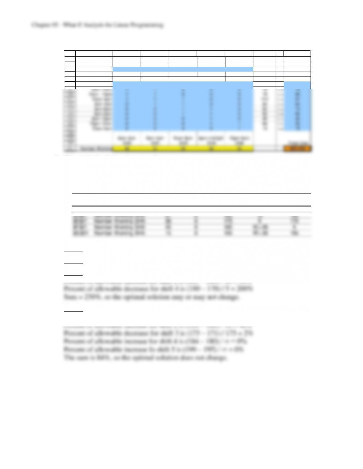
6am-2pm 8am-4pm Noon-8pm 4pm-midnight 10pm-6am
Shift Shift Shift Shift Shift Total Cost
Number Working 48 31 33 49 15 $30,150
5-10
c) Optimal Solution changes to:
3
4
5
6
7
8
9
10
11
12
13
14
15
16
17
18
19
20
21
B C D E F G H I J
6am-2pm 8am-4pm Noon-8pm 4pm-midnight 10pm-6am
Shift Shift Shift Shift Shift
Cost per Shift $170 $165 $175 $170 $195
Total Minimum
Time Period Shift W orks Time Period? (1=yes, 0= no) W orking Needed
6am-8am 1 0 0 0 0 48 >= 48
8am-10am 1 1 0 0 0 79 >= 79
10am- 12pm 1 1 0 0 0 79 >= 65
12pm-2pm 1 1 1 0 0 112 >= 87
2pm-4pm 0 1 1 0 0 64 >= 64
4pm-6pm 0 0 1 1 0 82 >= 73
6pm-8pm 0 0 1 1 0 82 >= 82
8pm-10pm 0 0 0 1 0 49 >= 43
10pm-12am 0 0 0 1 1 64 >= 52
12am-6am 0 0 0 0 1 15 >= 15
6am-2pm 8am-4pm Noon-8pm 4pm-midnight 10pm-6am
Shift Shift Shift Shift Shift Total Cost
Number Working 48 31 33 49 15 $30,305
d) The optimal solution does not change.
e) The optimal solution does not change.
f)
Variable Cells
Final Reduced Objective Allowable Allowable
Cell Name Value Cost Coefficient Increase Decrease
$C$21 Number Working Shift 48 0 170 1E+30 10
$D$21 Number Working Shift 31 0 160 10 160
$E$21 Number Working Shift 39 0 175 5 175
$F$21 Number Working Shift 43 0 180 1E+30 5
$G$21 Number Working Shift 15 0 195 1E+30 195
Part a) Optimal solution does not change (within allowable increase of $10).
Part b) Optimal solution does change (outside of allowable decrease of $5).
Part c)
Part d)
Percent of allowable decrease for shift 1 is (170 – 166) / 10 = 40%
5-11
Part e)
Percent of allowable increase for shift 1 is (173.40 – 170) / ∞ = 0%
g)
24
25
26
27
28
29
30
31
32
33
34
35
36
37
$185 48 31 39 43 15 $31,330
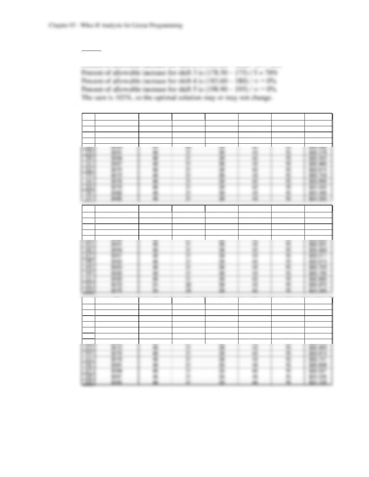
B C D E F G H
Cost per Shift 6am-2pm 8am-4pm Noon-8pm 4pm-midnight 10pm-6am Total
6am-2pm Shift Shift Shift Shift Shift Cost
48 31 39 43 15 $30,610
$155 54 25 39 43 15 $29,860
$158 54 25 39 43 15 $30,022
$161 48 31 39 43 15 $30,178
$164 48 31 39 43 15 $30,322
$167 48 31 39 43 15 $30,466
$170 48 31 39 43 15 $30,610
$173 48 31 39 43 15 $30,754
$176 48 31 39 43 15 $30,898
$179 48 31 39 43 15 $31,042
$182 48 31 39 43 15 $31,186
69
$190 48 31 33 49 15 $31,135
56
57
58
59
60
61
62
63
64
65
66
67
68
B C D E F G H
Cost per Shift 6am-2pm 8am-4pm Noon-8pm 4pm-midnight 10pm-6am Total
Noon-8pm Shift Shift Shift Shift Shift Cost
48 31 39 43 15 $30,610
$160 48 31 39 43 15 $30,025
$163 48 31 39 43 15 $30,142
$166 48 31 39 43 15 $30,259
$169 48 31 39 43 15 $30,376
$172 48 31 39 43 15 $30,493
$175 48 31 39 43 15 $30,610
$178 48 31 39 43 15 $30,727
$181 48 31 33 49 15 $30,838
$184 48 31 33 49 15 $30,937
$187 48 31 33 49 15 $31,036
5-12
85
$195 48 31 39 43 15 $31,255
72
73
74
75
76
77
78
79
80
81
82
83
84
B C D E F G H
Cost per Shift 6am-2pm 8am-4pm Noon-8pm 4pm-midnight 10pm-6am Total
4pm-midnight Shift Shift Shift Shift Shift Cost
48 31 39 43 15 $30,610
$165 48 31 33 49 15 $29,905
$168 48 31 33 49 15 $30,052
$171 48 31 33 49 15 $30,199
$174 48 31 33 49 15 $30,346
$177 48 31 39 43 15 $30,481
$180 48 31 39 43 15 $30,610
$183 48 31 39 43 15 $30,739
$186 48 31 39 43 15 $30,868
$189 48 31 39 43 15 $30,997
$192 48 31 39 43 15 $31,126
5.5 a) The optimal solution changes to
3
4
5
6
7
8
9
10
11
12
13
14
15
16
B C D E F G H
Office Shopping
Building Hotel Center
Net Present Value 45.2 70 50
($millions) Cumulative Cumulative
Capital Capital
Cumulative Capital Required ($millions) Spent Available
Now 40 80 90 24.299 <= 25
End of Year 1 100 160 140 45.000 <= 45
End of Year 2 190 240 160 65.000 <= 65
End of Year 3 200 310 220 80 <= 80
Office Shopping Total NPV
Building Hotel Center ($millions)
Participation Share 13.31% 6.12% 15.65% 18.12
b) The optimal solution does not change.
5-13
e) The optimal solution changes to
3
4
5
6
7
8
9
10
11
12
13
14
15
16
B C D E F G H
Office Shopping
Building Hotel Center
Net Present Value 40 70.2 49.8
($millions) Cumulative Cumulative
Capital Capital
Cumulative Capital Required ($millions) Spent Available
Now 40 80 90 20.645 <= 25
End of Year 1 100 160 140 41.290 <= 45
End of Year 2 190 240 160 61.935 <= 65
End of Year 3 200 310 220 80 <= 80
Office Shopping Total NPV
Building Hotel Center ($millions)
Participation Share 0.00% 25.81% 0.00% 18.12
f) The optimal solution changes to
3
4
5
6
7
8
9
10
11
12
13
14
15
16
B C D E F G H
Office Shopping
Building Hotel Center
Net Present Value 46 69 49
($millions) Cumulative Cumulative
Capital Capital
Cumulative Capital Required ($millions) Spent Available
Now 40 80 90 24.299 <= 25
End of Year 1 100 160 140 45.000 <= 45
End of Year 2 190 240 160 65.000 <= 65
End of Year 3 200 310 220 80 <= 80
Office Shopping Total NPV
Building Hotel Center ($millions)
Participation Share 13.31% 6.12% 15.65% 18.01
g) The optimal solution does not change.
h)
Variable Cells
Final Reduced O bjective Allowable Allowable
Cell Name Value Cost Coefficient Increase Decrease
$C$16 Participation Share Building 0.00% -4.85% 45 0.0485 1E+ 30
$D$16 Participation Share Hotel 16.50% 0.00% 70 0.4545 0.0543
$E$16 Participation Share Center 13.11% 0.00% 50 0.1389 0.3226
Constraints
Final Sh adow Constraint Allow able Allowable
Cell Name Value Price R.H. Side In crease Decrease
$F$9 Now Spent 25 0.0097 25 0.3049 4.3548
$F$10 End of Year 1 Spent 44.757 0.0000 45 1E+ 30 0.2427
$F$11 End of Year 2 Spent 60.583 0.0000 65 1E+ 30 4.4175
$F$12 End of Year 3 Spent 80 0.2233 80 0.7812 18.8889
Part a) Optimal solution changes (not within allowable increase of $48,500).
Part b) Optimal solution does not change (within allowable increase of $454,500).
5-14
Part e)
Part f)
Percentage of allowable increase for project 1 = (46 – 45) / 0.0485 = 2,062%
Part g)
i)
19
20
21
22
23
24
25
26
27
28
29
30
31
32
33
B C D E F
Net Present Value Participation
Project 1 (Office) Office Shopping Total NPV
($millions) Building Hotel Center ($millions)
0.00% 16.50% 13.11% 18.11
40 0.00% 16.50% 13.11% 18.11
41 0.00% 16.50% 13.11% 18.11
42 0.00% 16.50% 13.11% 18.11
43 0.00% 16.50% 13.11% 18.11
44 0.00% 16.50% 13.11% 18.11
45 0.00% 16.50% 13.11% 18.11
46 13.31% 6.12% 15.65% 18.23
47 13.31% 6.12% 15.65% 18.36
48 13.31% 6.12% 15.65% 18.49
49 13.31% 6.12% 15.65% 18.63
50 13.31% 6.12% 15.65% 18.76
5-15
36
37
38
39
40
41
42
43
44
45
46
47
48
49
50
B C D E F
Net Present Value Participation
Project 2 (Hotel) Office Shopping Total NPV
($millions) Building Hotel Center ($millions)
0.00% 16.50% 13.11% 18.11
65 13.31% 6.12% 15.65% 17.79
66 13.31% 6.12% 15.65% 17.85
67 13.31% 6.12% 15.65% 17.91
68 13.31% 6.12% 15.65% 17.97
69 13.31% 6.12% 15.65% 18.03
70 0.00% 16.50% 13.11% 18.11
71 0.00% 25.81% 0.00% 18.32
72 0.00% 25.81% 0.00% 18.58
73 0.00% 25.81% 0.00% 18.84
74 0.00% 25.81% 0.00% 19.10
75 0.00% 25.81% 0.00% 19.35
53
54
55
56
57
58
59
60
61
62
63
64
65
66
67
B C D E F
Net Present Value Participation
Project 3 (Shopping C.) Office Shopping Total NPV
($millions) Building Hotel Center ($millions)
0.00% 16.50% 13.11% 18.11
45 0.00% 25.81% 0.00% 18.06
46 0.00% 25.81% 0.00% 18.06
47 0.00% 25.81% 0.00% 18.06
48 0.00% 25.81% 0.00% 18.06
49 0.00% 25.81% 0.00% 18.06
50 0.00% 16.50% 13.11% 18.11
51 4.03% 12.90% 14.52% 18.25
52 13.31% 6.12% 15.65% 18.41
53 13.31% 6.12% 15.65% 18.56
54 13.31% 6.12% 15.65% 18.72
55 13.31% 6.12% 15.65% 18.88
5.6 The model Ep(x) is developed to identify a long-term management plan that satisfies the
legal requirements and optimizes PALCO’s operations and profitability. The model
5-16
The financial benefits of this study include an increase of over $398 million in present net
worth and of over $29 million in average yearly net revenues. Sustained-yield annual-
harvest levels have increased. The habitat mix is improved in accordance with political and
5.7 a) The decrease is within the allowable decrease, so the optimal production quantities stay
b) $0.30 is 0.30/0.65 = 46.2% of the allowable increase for steins.
$0.25 is 0.25/0.37 = 67.5% of the allowable decrease for plates.
c) 8 hours, or 480 minutes, is within the allowable decrease for molding, so the shadow
d) The shadow price for finishing ($0.28) is higher than the shadow price for molding
($0.22), so shifting minutes from molding to finishing would be beneficial, and would
e) 300. The shadow price is 0 because there is slack in this constraint. The shadow price
5.8 a) Optimal solution: produce no chocolate ice cream, 300 gallons of vanilla ice cream, and
75 gallons of banana ice cream. Total profit will be $341.25.
b) The optimal solution will change since $1.00 (an increase of $0.05) is outside the
c) The optimal solution will not change since $0.92 (a decrease of $0.03) is within the
d) The optimal solution will change. Since the change is within the allowable range, we
5-17
e) This increase is outside of the allowable increase so the total increase in profit with the
extra sugar can not be determined without re-solving. However, we know that the
f) The final value is 180 as shown in the E5 in the spreadsheet. The shadow price is 0
since we are using less milk than we have available (there is slack in the constraint).
The R.H.Side value is 200 as given in cell G5. The allowable increase is infinity since
5.9 a) The decrease is within the allowable decrease, so the optimal production quantities stay
the same. Total profit will decrease by ($50)(15) = $750 to $15,450.
b) $60 is 60/120 = 50% of the allowable decrease for tables.
d) The shadow price for finishing ($4.50) is higher than the shadow price for assembly
($2), so shifting minutes from assembly to finishing would be beneficial, and would
e) The shadow price is 0, and the allowable increase and decrease are 1E+30 (∞) and 400,
respectively. The shadow price is 0 because there is slack in this constraint. The
5.10 a) Let G = number of grandfather clocks produced
W = number of wall clocks produced
Maximize Profit = $300G + $200W
5-18
clocks per week.
c)
1
2
3
4
5
6
7
8
9
10
11
12
A B C D E F
Grandfather W all
Clock Clock
Unit Profit $300 $200
Hours Hours
Used Available
Assembly (David) 6 4 33 <= 40
Carving (LaDeana) 8 4 40 <= 40
Shipping (Lydia) 3 3 20 <= 20
Grandfather W all
Clock Clock Total Profit
Production 3.33 3.33 $1,667
Time Required
5-19
d) If the unit profit for grandfather clocks changes to $375, then the solution does not
change.
1
2
3
4
5
6
7
8
9
10
11
12
A B C D E F
Grandfather W all
Clock Clock
Unit Profit $375 $200
Hours Hours
Used Available
Assembly (David) 6 4 33 <= 40
Carving (LaDeana) 8 4 40 <= 40
Shipping (Lydia) 3 3 20 <= 20
Grandfather W all
Clock Clock Total Profit
Production 3.33 3.33 $1,917
Time Required
However, if the unit profit for wall clocks changes to $175 as well, then the optimal
solution does change (produce 5 grandfather clocks and 0 wall clocks).
1
2
3
4
5
6
7
8
9
10
11
12
A B C D E F
Grandfather W all
Clock Clock
Unit Profit $375 $175
Hours Hours
Used Available
Assembly (David) 6 4 30 <= 40
Carving (LaDeana) 8 4 40 <= 40
Shipping (Lydia) 3 3 15 <= 20
Grandfather W all
Clock Clock Total Profit
Production 5 0 $1,875
Time Required